MATH167R: Basic Definitions

Peter Gao

Warm-up: Getting to know each other

In groups of two or three, share:

Introduce yourself
Discuss what you think the following code does (feel free to try it out):

sides <- 1:6
rolls <- sample(sides, 100, replace = T)
print(sum(rolls == 1))

[1] 16

Overview of today

Basic definitions: objects, expressions, functions, data types
File paths and file management
R Markdown

Basic definitions

Review

“To understand computations in R, two slogans are helpful: Everything that exists is an object. Everything that happens is a function call.”

(Chambers, 2014)

We saw last class that we can use R to perform basic mathematical operations:

3 + 5

[1] 8

Expressions

We saw last class that we can use R to perform basic mathematical operations:

3 + 5

[1] 8

Definition: an expression is a symbol or a combination of symbols that evaluates to a value.

1 + 2

[1] 3

Objects

Definition: An object is created when R evaluates an expression. The object is accessible only by name.

An anonymous object gets deleted from the computer memory by a process called garbage collection.
A special object named .Last.value contains the value of the last evaluated expression (in console only).

Assignment

We saw last class that we can assign names to values:

x <- 1 + 2
x

[1] 3

Definition: Assignment is an operation to bind an object to name, using the symbol <-.

Note: = and <- are not generally equivalent. However, they are equivalent when they are used as assignment operators.

x = 1 + 2
x

[1] 3

Check your understanding: Assignment

What do you expect the output of the following chunks to be?

x <- 1
y <- x + 1
x <- 0
z <- y + 1
print(z)

a <- 1
b <- a + 1
b <- 2 * b
print(b)

Check your understanding: Assignment

What do you expect the output of the following chunks to be?

x <- 1
y <- x + 1
x <- 0
z <- y + 1
print(z)

[1] 3

a <- 1
b <- a + 1
b <- 2 * b
print(b)

[1] 4

Objects and data

We can use assignments to save values as named objects and perform math on the objects:

x <- 3
y <- 5
x + y

[1] 8

Today we’ll see that R can handle objects that are not numbers:

z <- "Hello"

Note: be careful because not all operations work with all types of data:

x + z

Error in x + z: non-numeric argument to binary operator

Atomic vectors

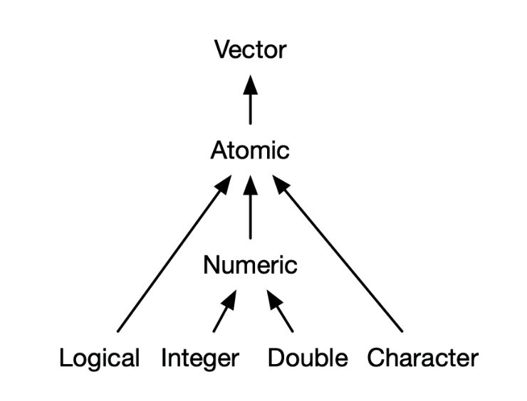
The most basic type of object in R used for storing values is the atomic vector. The four most common types of atomic vectors are:

logical: ex. TRUE or FALSE
integer: ex. 1, 2, 3, 4, …
double: ex. 3.1
character: ex. "Hello"

Integers and doubles are both also called numeric vectors.

Atomic vectors

from Advanced R, Hadley Wickham.

Atomic vectors

example_lgc <- T
example_int <- 1L

The typeof function can be used to get the data type of an object.

typeof(example_lgc)

[1] "logical"

typeof(example_int)

[1] "integer"

Atomic vectors

example_dbl <- 1.0
example_chr <- "Hello"

The typeof function can be used to get the data type of an object.

typeof(example_dbl)

[1] "double"

typeof(example_chr)

[1] "character"

Coercion

You can explicitly change the type of an object:

as.numeric(example_lgc)

[1] 1

as.numeric(example_chr)

[1] NA

Coercion

When elements of different types are mixed in an atomic vector, R automatically converts all of them to the same type.

Order of precedence, from the highest to the lowest: character, numeric, integer, logical.

c(TRUE, "hello", 1)

[1] "TRUE"  "hello" "1"

Special values

Value	Usual meaning
`NA`	Missing values
`NaN`	a computed value that is not a number
`NULL`	an object with no value
`-Inf` and `Inf`	a computed value that is large (or large and negative)

Environment

When R evaluates an expression such as x + 1, how does R locate the object associated with the name x?

During an assignment, the binding between an object and its name is stored in an environment.

When R starts, a global environment (sometimes called a workspace) is created; every subsequent assignment that takes place at the command prompt adds objects to this environment.

Environment

We will see later that we can enter local environments within the global environment and define objects that are confined to these local environments.

The ls() command displays object in the current global environment.

To remove objects, we can use the rm() command.

Operators

An operator is a symbol that tells the compiler to perform specific mathematical or logical operations.

Types of operators:

Assignment operators
Arithmetic operators
Logical operators
Relational operators

Arithmetic Operators

Operator	Operation	Example	Result
`+`	Addition	`> 3 + 4`	`[1] 7`
`-`	Subtraction	`> 3 - 4`	`[1] -1`
`*`	Multiplication	`> 3 * 4`	`[1] 12`
`/`	Division	`> 3 / 4`	`[1] 0.75`

Arithmetic Operators

Operator	Operation	Example	Result
`^` or `**`	Exponentiation	`> 3 ^ 4`	`[1] 81`
`%%`	Modulo	`> 3 %% 4`	`[1] 3`

Logical Operators

Operator	Operation	Example	Result
`&`	AND	`> TRUE & FALSE`	`[1] FALSE`
`\|`	OR	`> TRUE \| FALSE`	`[1] TRUE`
`!`	NOT	`> !TRUE`	`[1] FALSE`

Relational Operators

Operator	Operation	Example	Result
`>`	greater than	`> 2 > 1`	`[1] TRUE`
`>=`	greater than or equal to	`> 2 >= 1`	`[1] TRUE`
`==`	equal	`> 2 == 1`	`[1] FALSE`
`<=`	less than or equal to	`> 2 <= 1`	`[1] FALSE`
`<`	less than	`> 2 < 1`	`[1] FALSE`
`!=`	not equal to	`> 2 != 1`	`[1] TRUE`

Check your understanding: Operators

TRUE & FALSE & TRUE
TRUE & (FALSE | TRUE)
1 < 4
(1 < 4) & (3 > 4)

Check your understanding: Operators

Answers:

TRUE & FALSE & TRUE

[1] FALSE

TRUE & (FALSE | TRUE)

[1] TRUE

1 < 4

[1] TRUE

(1 < 4) & (3 > 4)

[1] FALSE

File management

The working directory

The working directory is a folder where files are retrieved from or saved to by default.
The command getwd() gets the working directory, which usually is:
- /Users/USERNAME on Apple
- C:\Users\USERNAME on Windows
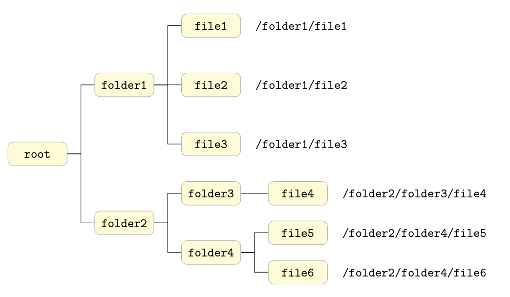
Files on a computer are grouped into folders, which are organized in a hierarchy.
The absolute pathname of a file describes its location in the hierarchy.

Relative pathnames

The relative pathname of a file specifies its location relative to the working directory.

The command setwd() sets the working directory for the current R session.

getwd()
setwd("/Users/pgao/Desktop")

On Windows, add C: to the beginning of the absolute pathname.

getwd()
setwd("C:/Documents/")

Example file structure

Project-based workflow

In this class, I encourage you to organize all your code/assignments/files into a single MATH167R folder.

Once you create this folder, you can create an RStudio Project, which will create a file that tells RStudio that all the code in the folder is associated with a single project.

Any code in the project folder assumes that the working directory is the project root directory. This ensures that the project can be moved around your computer or onto another computer and none of the paths will break. This solves the issue of everyone having differing home directories.

Project-based workflow

Create a folder called MATH167R on your computer.
In RStudio, click File > New Project > Existing Directory and select your MATH167R folder. This will create an .Rproj file that indicates to R where the working directory for this project should be.
(Optional) Create a shortcut to this .Rproj file to easily open your work for this class.

Example file structure for MATH167R

MATH167R
├── labs
│   ├── 01_lab.R
│   └── 02_lab.R
├── checkins
│   ├── 01_checkin.R
│   └── 02_checkin.R
├── project
│   └── data
│       └── trees.csv
└── exams

Naming files

Tips from Jenny Bryan:

machine readable
human readable
plays well with default ordering

Naming files

Bad:

newfinal2actualFINALnew.docx
my first lab.R
stuff.R

Better:

01_lab1.Rmd
analysis_functions.R
2020-01-08_labWriteup.Rmd

R Markdown

R Markdown files (see examples here)

Combine code, output, and writing
Self-contained analyses
Creates HTML, PDF, slides (like these!), webpages, …
will be required for assignments

Your first RMarkdown file

Open this link. At the top right corner of this website, click “Code” to get the code for this document.

At the top of the file, you should see the following header:

---
title: "Check-in 1: R Markdown"
author: "YOUR NAME HERE"
date: "2024-01-29"
output: html_document
---

This header contains metadata about the document that follows: the name of the file, the author, the date, and what kind of output it will create. Highlight all this code and copy it to your clipboard.

Your first RMarkdown file

In RStudio, click File > New File > R Markdown > OK to accept all default options. A new .Rmd file should open. Replace everything in the new file with your copied code.

---
title: "Check-in 1: R Markdown"
author: "YOUR NAME HERE"
date: "2024-01-29"
output: html_document
---

This header contains metadata about the document that follows: the name of the file, the author, the date, and what kind of output it will create.

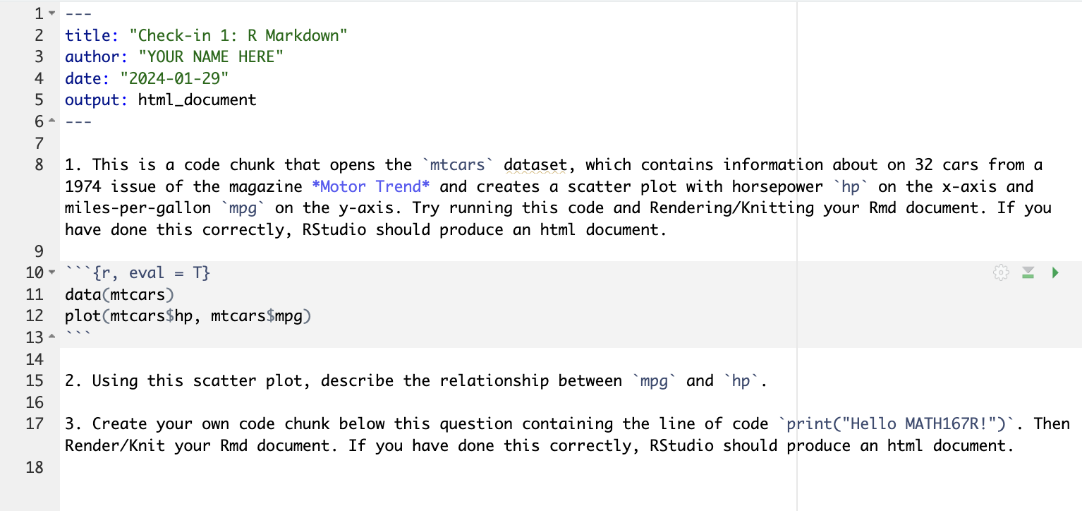
Source Editor

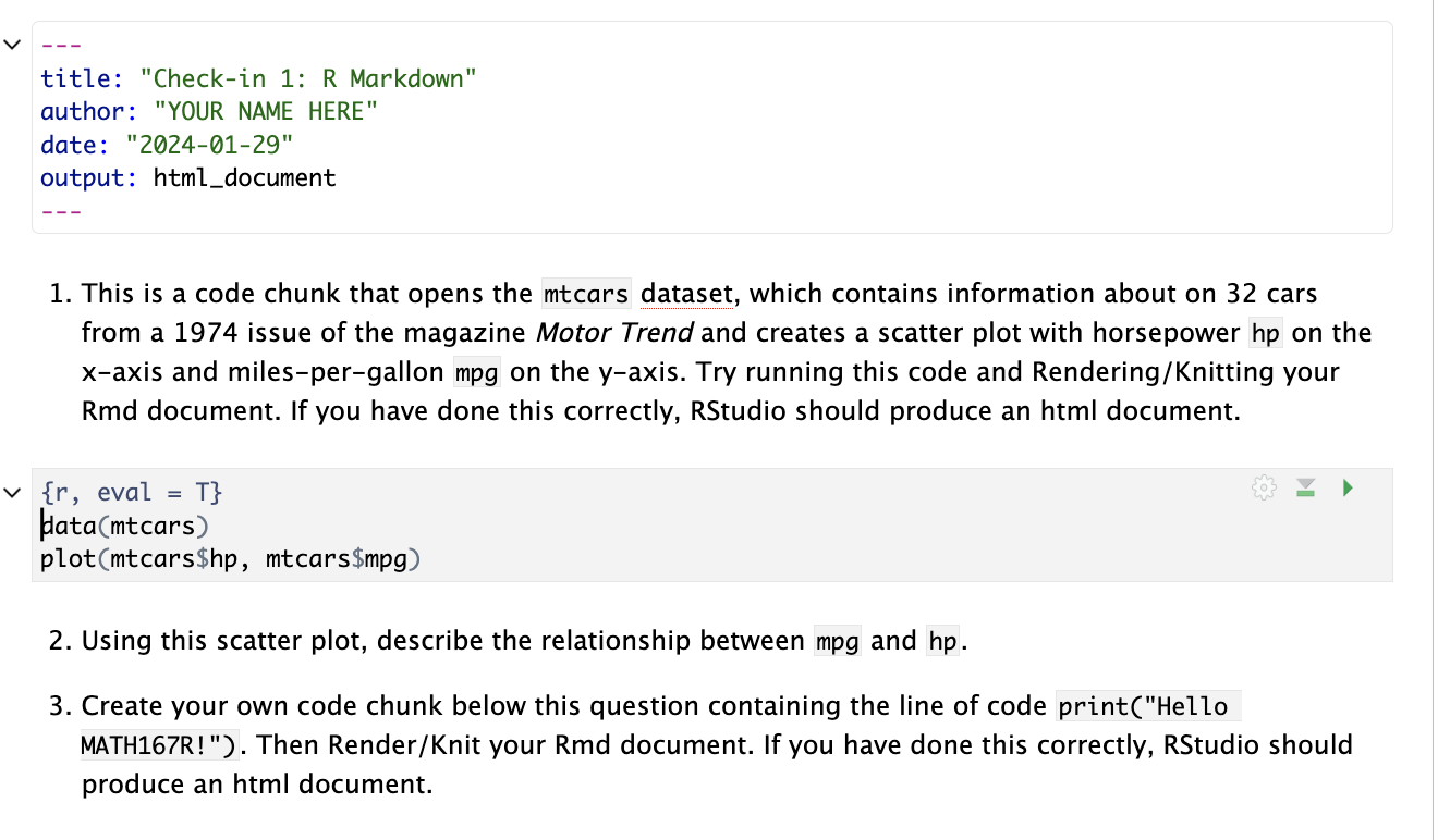
Visual Editor

Code chunks

Code chunks contain R code that is evaluated when you render your R Markdown report. You can insert a code chunk by clicking Insert > Code Chunk or by typing the chunk delimiters ```{r} and ``` .

Chunk output can be customized with optional arguments set in the {} of a chunk header, as we will see in Lab 01.

R Markdown (and directory weirdness)

R Markdown handles all the tricky file management–just put the file you want to access in the same folder as your .Rmd file
This can be confusing/frustrating—patience is key!

R Markdown

Remember the following:

R Markdown produces fully reproducible reports – each time you render, you run the analysis from the beginning of the document.
Code goes in chunks, while the explanation/narrative goes outside of chunks
RStudio now provides a visual editor for a familiar / Google docs-like editing experience

Check-in 1

Not due for a while, but in your interest to do this ASAP to make sure R Markdown is working!