MATH167R: Advanced visualizations
Overview of today
- Visualizing spatial data
- Animations
- Project work time
Example: PM 2.5 data
The EPA provides daily data on air quality for monitoring stations across the country, which you can download here. The below code downloads a subset of this data from the course website for the pollutant PM 2.5 (atmospheric particulate matter with a diameter of less than 2.5 micrometers) and AQI for 2023.
Example: PM 2.5 data
| Date | Source | Site ID | POC | Daily Mean PM2.5 Concentration | UNITS | DAILY_AQI_VALUE | Site Name | DAILY_OBS_COUNT | PERCENT_COMPLETE | AQS_PARAMETER_CODE | AQS_PARAMETER_DESC | CBSA_CODE | CBSA_NAME | STATE_CODE | STATE | COUNTY_CODE | COUNTY | SITE_LATITUDE | SITE_LONGITUDE |
|---|---|---|---|---|---|---|---|---|---|---|---|---|---|---|---|---|---|---|---|
| 01/01/2023 | AQS | 060010007 | 3 | 3.7 | ug/m3 LC | 15 | Livermore | 1 | 100 | 88101 | PM2.5 - Local Conditions | 41860 | San Francisco-Oakland-Hayward, CA | 06 | California | 001 | Alameda | 37.68753 | -121.7842 |
| 01/02/2023 | AQS | 060010007 | 3 | 2.7 | ug/m3 LC | 11 | Livermore | 1 | 100 | 88101 | PM2.5 - Local Conditions | 41860 | San Francisco-Oakland-Hayward, CA | 06 | California | 001 | Alameda | 37.68753 | -121.7842 |
| 01/03/2023 | AQS | 060010007 | 3 | 3.6 | ug/m3 LC | 15 | Livermore | 1 | 100 | 88101 | PM2.5 - Local Conditions | 41860 | San Francisco-Oakland-Hayward, CA | 06 | California | 001 | Alameda | 37.68753 | -121.7842 |
| 01/04/2023 | AQS | 060010007 | 3 | 2.7 | ug/m3 LC | 11 | Livermore | 1 | 100 | 88101 | PM2.5 - Local Conditions | 41860 | San Francisco-Oakland-Hayward, CA | 06 | California | 001 | Alameda | 37.68753 | -121.7842 |
| 01/05/2023 | AQS | 060010007 | 3 | 4.7 | ug/m3 LC | 20 | Livermore | 1 | 100 | 88101 | PM2.5 - Local Conditions | 41860 | San Francisco-Oakland-Hayward, CA | 06 | California | 001 | Alameda | 37.68753 | -121.7842 |
| 01/06/2023 | AQS | 060010007 | 3 | 9.2 | ug/m3 LC | 38 | Livermore | 1 | 100 | 88101 | PM2.5 - Local Conditions | 41860 | San Francisco-Oakland-Hayward, CA | 06 | California | 001 | Alameda | 37.68753 | -121.7842 |
Example: PM 2.5 data
     Date              Source            Site ID               POC
 Length:51541       Length:51541       Length:51541       Min.   : 1.000
 Class :character   Class :character   Class :character   1st Qu.: 2.000
 Mode  :character   Mode  :character   Mode  :character   Median : 3.000
                                                          Mean   : 2.634
                                                          3rd Qu.: 3.000
                                                          Max.   :12.000

 Daily Mean PM2.5 Concentration    UNITS           DAILY_AQI_VALUE
 Min.   : -3.000                Length:51541       Min.   :  0.00
 1st Qu.:  3.900                Class :character   1st Qu.: 16.00
 Median :  6.500                Mode  :character   Median : 27.00
 Mean   :  7.823                                   Mean   : 30.64
 3rd Qu.: 10.000                                   3rd Qu.: 42.00
 Max.   :235.100                                   Max.   :285.00

  Site Name         DAILY_OBS_COUNT PERCENT_COMPLETE AQS_PARAMETER_CODE
 Length:51541       Min.   :1       Min.   :100      Min.   :88101
 Class :character   1st Qu.:1       1st Qu.:100      1st Qu.:88101
 Mode  :character   Median :1       Median :100      Median :88101
                    Mean   :1       Mean   :100      Mean   :88177
                    3rd Qu.:1       3rd Qu.:100      3rd Qu.:88101
                    Max.   :1       Max.   :100      Max.   :88502

 AQS_PARAMETER_DESC   CBSA_CODE      CBSA_NAME          STATE_CODE
 Length:51541       Min.   :12540   Length:51541       Length:51541
 Class :character   1st Qu.:31080   Class :character   Class :character
 Mode  :character   Median :40140   Mode  :character   Mode  :character
                    Mean   :35282
                    3rd Qu.:41860
                    Max.   :49700
                    NA's   :3920
    STATE           COUNTY_CODE           COUNTY          SITE_LATITUDE
 Length:51541       Length:51541       Length:51541       Min.   :32.58
 Class :character   Class :character   Class :character   1st Qu.:34.21
 Mode  :character   Mode  :character   Mode  :character   Median :36.60
                                                          Mean   :36.38
                                                          3rd Qu.:37.97
                                                          Max.   :41.76

 SITE_LONGITUDE
 Min.   :-124.2
 1st Qu.:-121.5
 Median :-119.8
 Mean   :-119.8
 3rd Qu.:-118.2
 Max.   :-115.5
Warm-up: PM 2.5 data
Work with the people around you to identify:
- Where and when was the highest
DAILY_AQI_VALUEobserved in 2023? - Which site had the highest median
DAILY_AQI_VALUEin 2023? - How many monitoring sites are in Santa Clara County?
- What is the name of the site in this dataset that is closest to SJSU’s campus?
- What is the median
DAILY_AQI_VALUEfor this site in 2023?
Warm-up: PM 2.5 data
Answers:
- Yreka on August 28 (AQI = 285)
- Cortina Indian Rancheria
- 3
- San Jose - Jackson
- 29
Data wrangling
Note that the Date variable is a character–we can convert this into a Date class object using the lubridate package.
      Date               Source            Site ID               POC
 Min.   :2023-01-01   Length:51541       Length:51541       Min.   : 1.000
 1st Qu.:2023-03-26   Class :character   Class :character   1st Qu.: 2.000
 Median :2023-06-21   Mode  :character   Mode  :character   Median : 3.000
 Mean   :2023-06-23                                         Mean   : 2.634
 3rd Qu.:2023-09-18                                         3rd Qu.: 3.000
 Max.   :2023-12-31                                         Max.   :12.000

 Daily Mean PM2.5 Concentration    UNITS           DAILY_AQI_VALUE
 Min.   : -3.000                Length:51541       Min.   :  0.00
 1st Qu.:  3.900                Class :character   1st Qu.: 16.00
 Median :  6.500                Mode  :character   Median : 27.00
 Mean   :  7.823                                   Mean   : 30.64
 3rd Qu.: 10.000                                   3rd Qu.: 42.00
 Max.   :235.100                                   Max.   :285.00

  Site Name         DAILY_OBS_COUNT PERCENT_COMPLETE AQS_PARAMETER_CODE
 Length:51541       Min.   :1       Min.   :100      Min.   :88101
 Class :character   1st Qu.:1       1st Qu.:100      1st Qu.:88101
 Mode  :character   Median :1       Median :100      Median :88101
                    Mean   :1       Mean   :100      Mean   :88177
                    3rd Qu.:1       3rd Qu.:100      3rd Qu.:88101
                    Max.   :1       Max.   :100      Max.   :88502

 AQS_PARAMETER_DESC   CBSA_CODE      CBSA_NAME          STATE_CODE
 Length:51541       Min.   :12540   Length:51541       Length:51541
 Class :character   1st Qu.:31080   Class :character   Class :character
 Mode  :character   Median :40140   Mode  :character   Mode  :character
                    Mean   :35282
                    3rd Qu.:41860
                    Max.   :49700
                    NA's   :3920
    STATE           COUNTY_CODE           COUNTY          SITE_LATITUDE
 Length:51541       Length:51541       Length:51541       Min.   :32.58
 Class :character   Class :character   Class :character   1st Qu.:34.21
 Mode  :character   Mode  :character   Mode  :character   Median :36.60
                                                          Mean   :36.38
                                                          3rd Qu.:37.97
                                                          Max.   :41.76

 SITE_LONGITUDE
 Min.   :-124.2
 1st Qu.:-121.5
 Median :-119.8
 Mean   :-119.8
 3rd Qu.:-118.2
 Max.   :-115.5
Wildfire season 2023
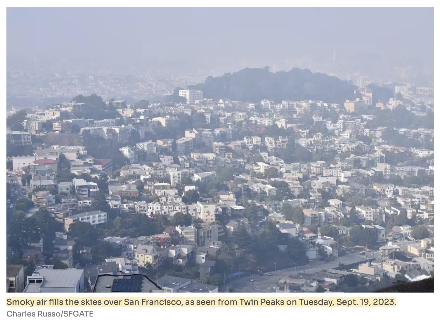
Wildfire season 2023
Working with spatial data
We can’t get an idea of how air quality varies over space using univariate summaries like these. Ideally, we could plot the PM 2.5 or AQI measurements on a map of California.
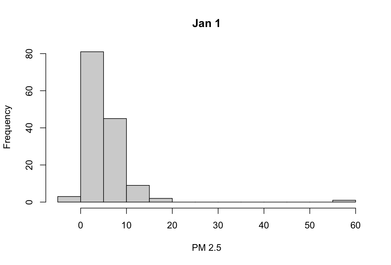
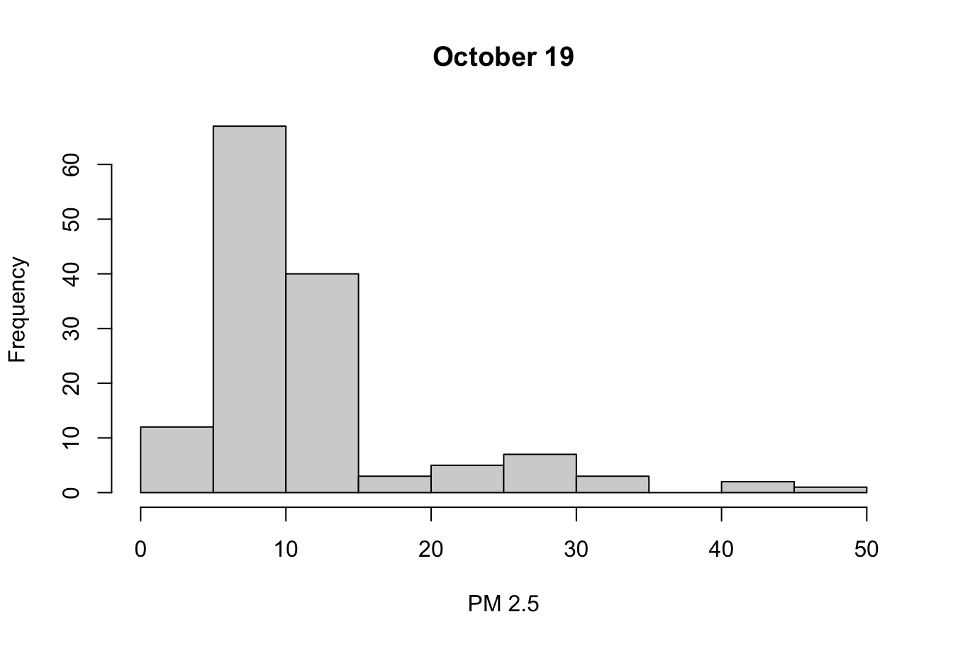
Naively working with latitude/longitude
Naively working with latitude/longitude
Compare with January 1:
Naively working with latitude/longitude
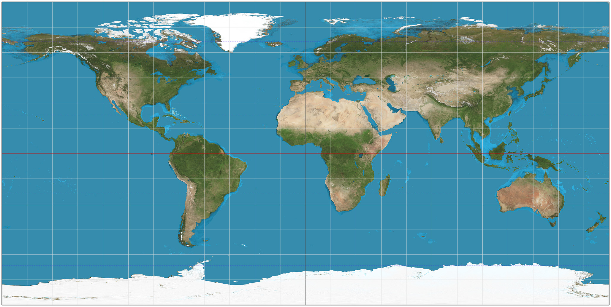
We can only get so far just treating longitude and latitude as x and y. In particular, near the poles, we will get large amounts of distortion:
Simple features
Simple Features is a set of standards for storing and accessing geographic data.
Geographic data typically consist of geometries such as points, lines, and polygons
In R, the most popular package for working with simple features data is
sf.Working with spatial data can be extremely memory intensive, so care is needed.
Converting data to simple features object
When each row in our data frame refers to a point with longitude and latitude, we can use the st_as_sf function to convert our data frame to an sf object.
Converting data to simple features object
Simple feature collection with 6 features and 18 fields
Geometry type: POINT
Dimension: XY
Bounding box: xmin: -122.2823 ymin: 37.68753 xmax: -121.7842 ymax: 39.76168
Geodetic CRS: WGS 84
# A tibble: 6 × 19
Date Source `Site ID` POC Daily Mean PM2.5 Con…¹ UNITS DAILY_AQI_VALUE
<date> <chr> <chr> <dbl> <dbl> <chr> <dbl>
1 2023-09-19 AQS 060010007 3 21.7 ug/m… 71
2 2023-09-19 AQS 060010009 3 27.9 ug/m… 84
3 2023-09-19 AQS 060010011 3 29.6 ug/m… 88
4 2023-09-19 AQS 060010012 3 33.3 ug/m… 96
5 2023-09-19 AQS 060010015 3 25.7 ug/m… 80
6 2023-09-19 AQS 060070008 3 7.1 ug/m… 30
# ℹ abbreviated name: ¹`Daily Mean PM2.5 Concentration`
# ℹ 12 more variables: `Site Name` <chr>, DAILY_OBS_COUNT <dbl>,
# PERCENT_COMPLETE <dbl>, AQS_PARAMETER_CODE <dbl>, AQS_PARAMETER_DESC <chr>,
# CBSA_CODE <dbl>, CBSA_NAME <chr>, STATE_CODE <chr>, STATE <chr>,
# COUNTY_CODE <chr>, COUNTY <chr>, geometry <POINT [°]>Visualizing point data
We can easily visualize this data now using the geom_sf() function, which automatically handles sf objects.
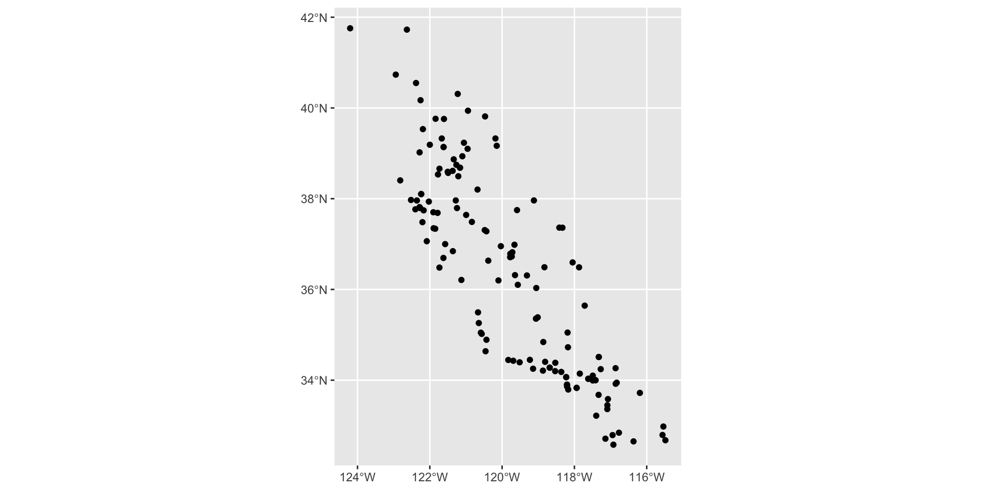
Visualizing point data
We can add a basemap by downloading the outline of California from the tigris package.
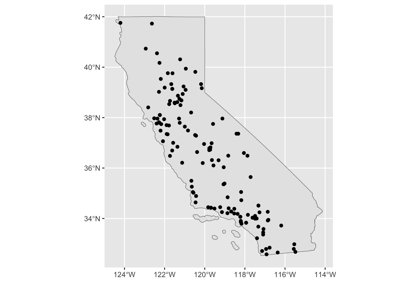
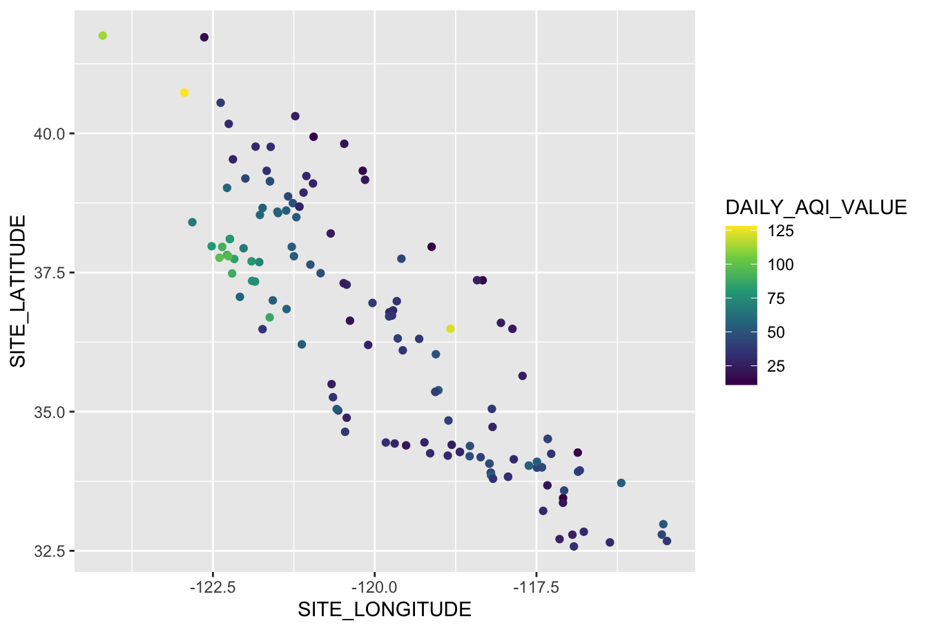
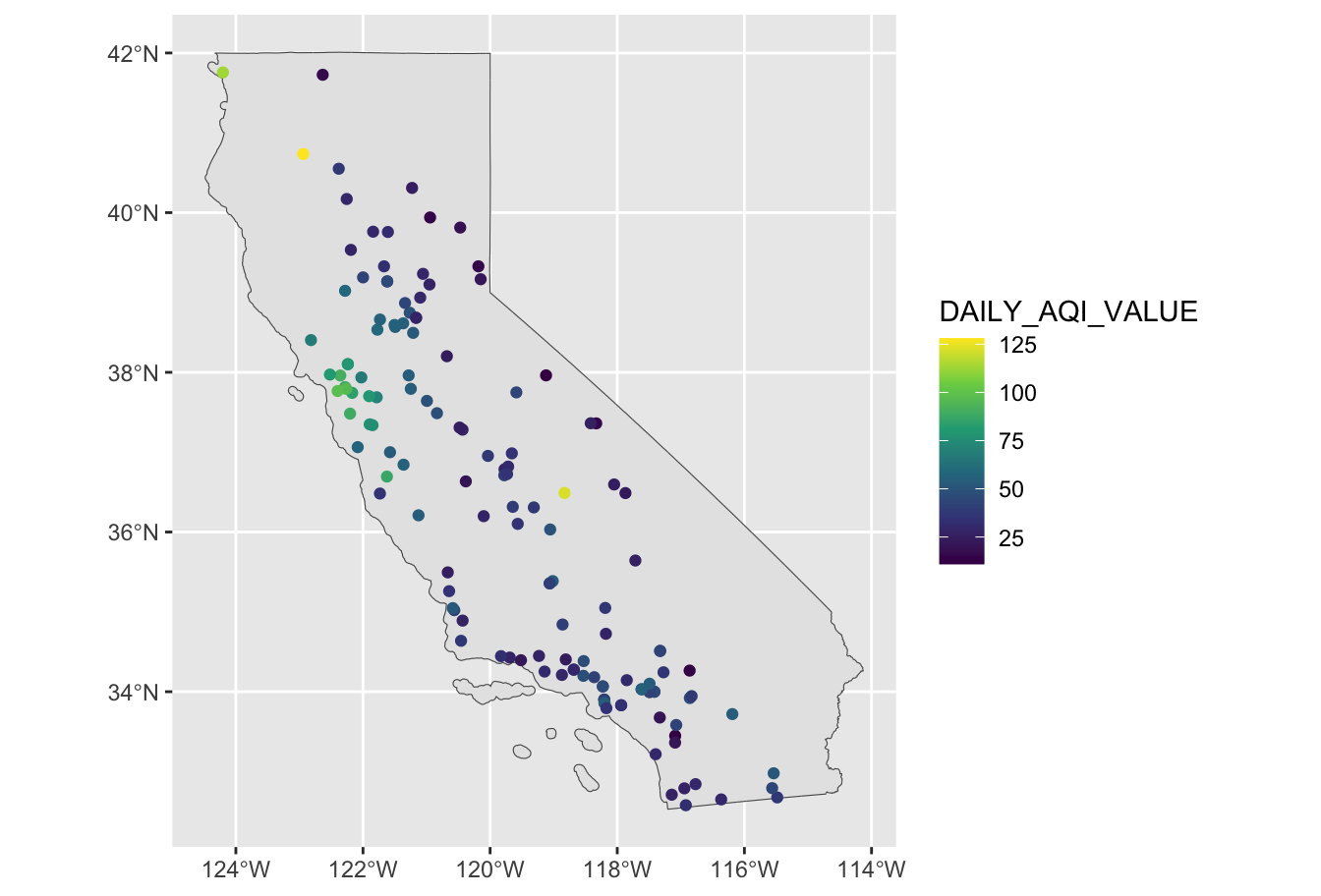
Visualizing point data
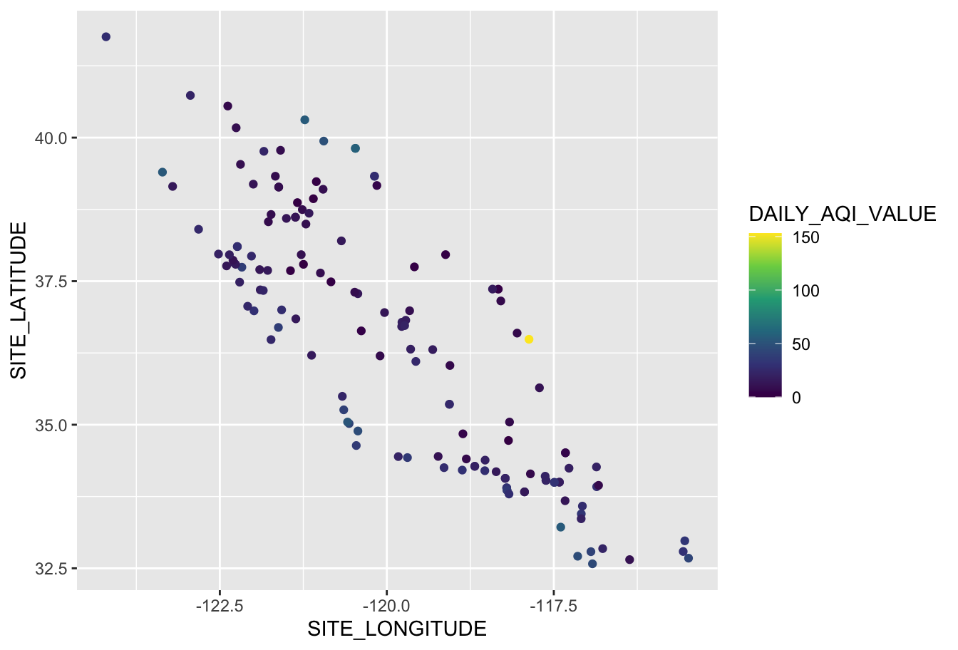
We can then adjust the color to show DAILY_AQI_VALUE and also change the color scale:
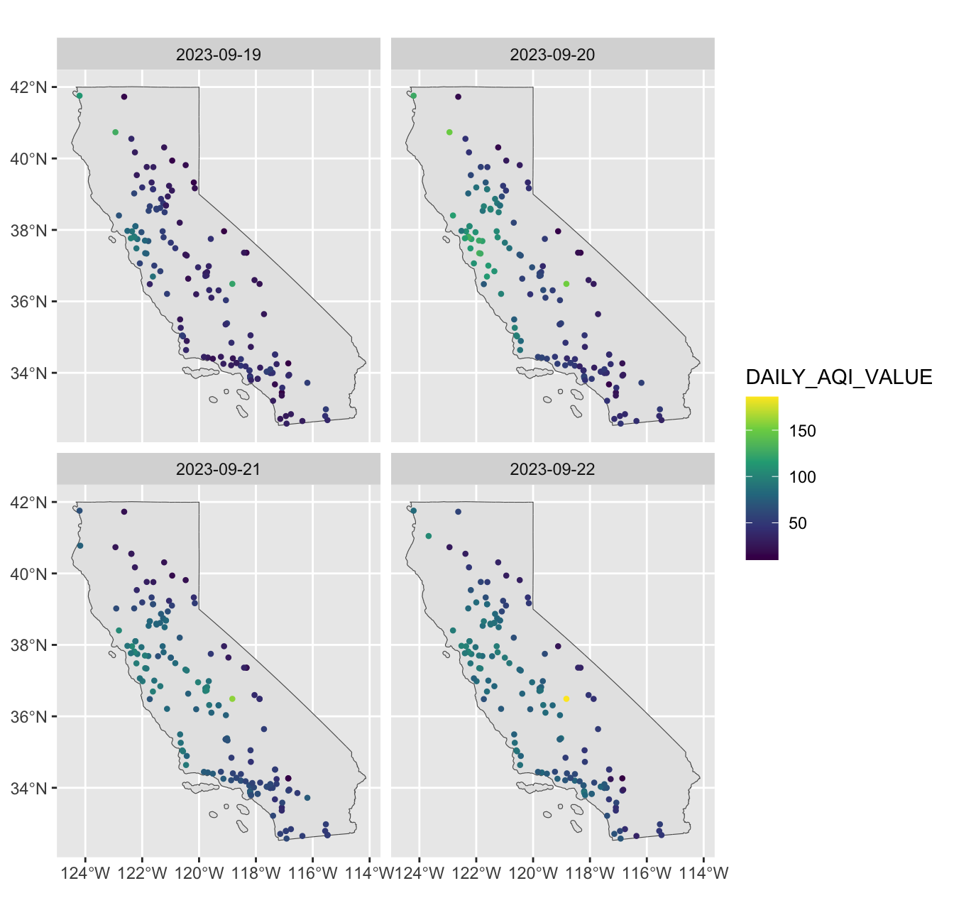
Exercise
How do we create the following plot?
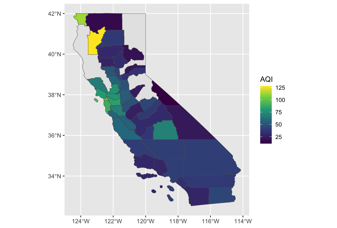
Spatial Polygon data
The AQI data we downloaded also contains county information. We can compute county level mean AQI using group_by and summarize:
Spatial Polygon data
We can then create a county-level polygon map by downloading county-level boundaries using tigris.
Spatial Polygon data
Animation with gganimate
The gganimate package provides tools for animating ggplot visualizations:
Animation with gganimate
ggplot(gapminder, aes(gdpPercap, lifeExp, size = pop, colour = country)) +
  geom_point(alpha = 0.7, show.legend = FALSE) +
  scale_colour_manual(values = country_colors) +
  scale_size(range = c(2, 12)) +
  scale_x_log10() +
  facet_wrap(~continent) +
  # Here comes the gganimate specific bits
  labs(title = 'Year: {frame_time}',
       x = 'GDP per capita',
       y = 'life expectancy') +
  transition_time(year) +
  ease_aes('linear')
Animation with gganimate
Animation with gganimate
pm_2_5 <- readr::read_csv("https://math167r-s24.github.io/static/CA_PM2_5_2023.csv")
pm_2_5 <- pm_2_5 |>
  mutate(Date = mdy(Date)) |>
  filter(month(Date) == 9)
ggplot() +
  geom_sf(data = CA_sf) +
  geom_point(data = pm_2_5,
             mapping = aes(
               x = SITE_LONGITUDE,
               y = SITE_LATITUDE,
               color = DAILY_AQI_VALUE
             )) +
  scale_color_viridis_c() +
  # Here comes the gganimate specific bits
  labs(title = "Date: {frame_time}") +
  transition_time(Date) +
  ease_aes('linear')
Takeaways
Packages like
sfandgganimateare complex and frequently changing – but extendggplotfor new types of data and visualizations.Don’t need to memorize these packages’ functions: get comfortable with documentation.
Be creative and challenge yourself–don’t limit yourself to the visuals we’ve created in class.
Other sources of spatial data
Final project
Instructions on the course website.