[1] 55MATH167R: Environment and Scope
Overview of today
- Environments and scope (based on Advanced R by Hadley Wickham)
- Lab time
Function composition
In mathematics, function composition is an operation that combines functions:
For example, if \(f(x) = x^2\) and \(g(x)=x+2\), what is \(f(g(x))\)?
Throughout this class we have been composing functions:
Function structure in R
Most functions in R have three parts:
formals(): the list of formal argumentsbody(): the code inside the functionenvironment(): the data structure that determines how objects and values are found when evaluating the function
Environments and scoping
Previously, we talked about assignment in R, which binds names to values.
Today we’ll talk about scoping, which involves finding a value associated with a name.
Exercise: What will the following code return?
[1] 10Environments and scoping
Exercise: What about this code?
[1] 20Lexical scoping
R generally uses lexical scoping meaning that a function accesses values of names based on how the function is defined and not how it is called.
Name masking
Name masking: names defined within a function mask names defined outside the function.
Exercise: What will the following code return?
[1] 1 2[1] 10Name masking
Now, y is a free variable, meaning that it is not defined as a formal argument or declared in the body of the function?
Exercise: What will the following code return?
[1] 1 20[1] 10Free variables
Lexical scoping means that free variables are searched for in the environment where the function is defined.
Environments
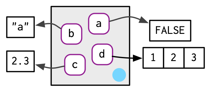
An environment is a collection of pairs of symbols (names) and values.
We can think of environments as simply bags of names bound to values (figure from Advanced R)

Environments
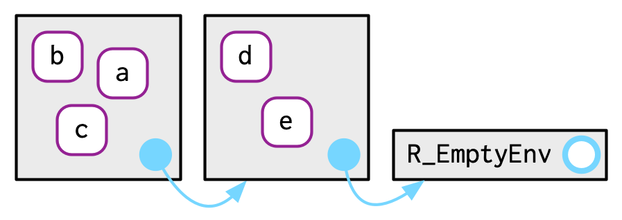
Environments are organized hierarchically: Every environment has a parent and may have one or multiple children.
There is one environment without a parent: the empty environment.

The global environment
When we work in RStudio and interact with the console, we are generally working in the global environment. The global environment is often called the workspace.
When we try to access a variable in the console (or click Run when editing an R Markdown document), we are working in the global environment.
Package environments
Whenever we load a package with library() we add a parent to the global environment:

We can see the current search path using the search() function.
Searching for a value
Suppose we are looking for a value for a given symbol used in a function.
- First, the search begins within the body of the function.
- Next, if the value is not found in the body, the search continues in the function’s environment (where it was defined).
- If the value is not found there, the search continues in the parent environment.
- The search continues up the sequence of parents until the empty environmnet is reached at which point we throw an error.
Example
Exercise: What will the following code return?
[1] 15Example
Exercise: What will the following code return?
[1] 15Example
Exercise: What will the following code return?
[1] 202Knitting/Rendering an R Markdown document
When you open RStudio, you are working in a (new) global environment.
When we click Run within RStudio, you are working in this same global environment.
However, when you knit an R Markdown document, you are essentially starting a new global environment, so you cannot access anything in your current workspace.
This ensures that the R Markdown document is self-contained and has everything that one would need to reproduce your results.
A fresh start: function execution
Each time you execute a function by calling it, a temporary environment is created.
Exercise: What will the following code return?
[1] 1[1] 1Super assignment
The <<- operator doesn’t create a variable in the current environment. It looks for a matching name in the parent environments. If it finds one, it updates that variable. If it doesn’t, it creates a variable in the global environment.
Practical tips
Remember:
Name masking: names defined within a function mask names defined outside the function.
Free variables: Free variables are searched for first in the environment where the function is defined.
Knitting an R Markdown document: R Markdown documents are self-contained, so when you knit, you cannot access anything in the global environment you were working in.
Function execution environments: Function execution environments are generally temporary, so whatever happens within a function does not affect the global environment.