[1] 4 3 6 5 1 7 9 9 6 8MATH167R: Simulations
Overview of today
- Random variables in R
- The
r,p,d, andqfunctions replicate()- Writing simulations
Random variables in R
We have already seen a number of functions for generating random variables such as sample() and rnorm().
Today, we will expand on these functions and related functions for studying random variables and begin using them to write various simulations.
Random variables in R
Remember that we can use the sample() function as follows to draw at random from a finite set with and without replacement:
What if we want to generate \(n\) samples from a normal distribution? Or a binomial distribution?
Simulating a coin-flipping game
Can we write code to simulate this game?

Simulating a coin-flipping game
Simulating a coin-flipping game
What if we want to simulate this game many times? One approach is to wrap our code in a function, which we can run many times.
Simulating a coin-flipping game
run_one_sim <- function(seed, n) {
  set.seed(seed)
  flips <- sample(x = c("H", "T"), size = n, replace = T)
  HH_score <- 0
  HT_score <- 0
  for (i in 2:n) {
    if (flips[i-1] == "H" & flips[i] == "H") {
      HH_score <- HH_score + 1
    }
    if (flips[i-1] == "H" & flips[i] == "T") {
      HT_score <- HT_score + 1
    }
  }
  return(list(HH = HH_score, HT = HT_score))
}
# run 100000 simulations with n = 100
results <- lapply(1:10000, run_one_sim, n = 100)

HH_scores <- sapply(results, function(x) x$HH)
HT_scores <- sapply(results, function(x) x$HT)
Simulating a coin-flipping game
Simulating a coin-flipping game
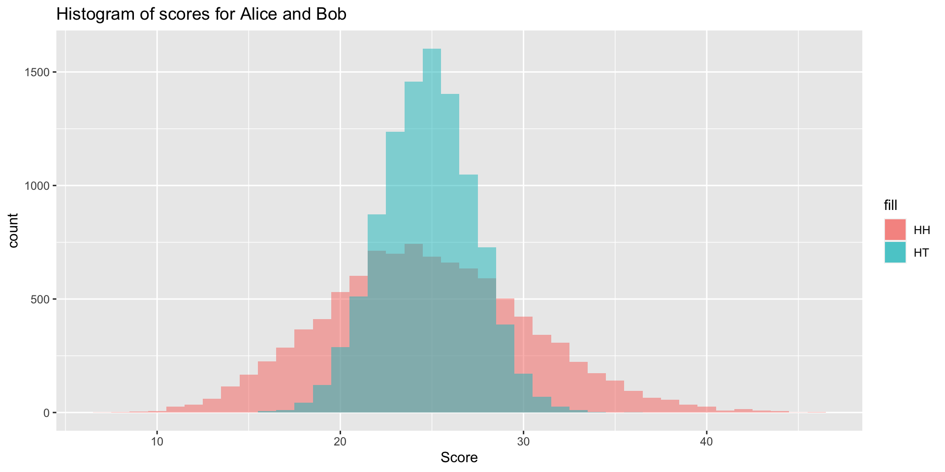
Why does Bob win more often? Intuitively, both “HH” and “HT” are equally likely when we flip a fair coin twice.
Simulating a coin-flipping game
Here’s a histogram of Alice and Bob’s scores across the simulations. What do you notice? How might this explain our results?

Simulating a coin-flipping game
The r, p, d, and q functions
What if we want to generate \(n\) samples from a normal distribution? Or a binomial distribution?
R provides functions for working with a variety of probability distributions. For most distributions, there are four functions: r, p, d, and q. As an example, let’s look at the normal distribution.
rnorm() can be used to generate n random observations from a normal distribution:
The r, p, d, and q functions
pnorm() can be used to compute the distribution function at a value q. In other words, if \(Z\) is a standard normal, pnorm returns the value of \[F(q)= P\left(Z \leq \frac{q-\mu}{\sigma}\right)\]
The r, p, d, and q functions
qnorm() can be used to compute the quantile function at a percentile p. In other words, if \(Z\) is a standard normal the quantile function returns the value \(x\) such that \[P\left(Z\leq \frac{x-\mu}{\sigma}\right)=p\]
The r, p, d, and q functions
dnorm() can be used to compute the density function at a value x: \[ f(x)={\frac {1}{\sigma {\sqrt {2\pi }}}}\exp\left\{-{\frac {1}{2}}\left({\frac {x-\mu }{\sigma }}\right)^{2}\right\}\]
Exercise
Create a histogram of 1000 samples from a normal distribution with mean 10 and standard deviation 20.
Exercise
Suppose we perform a two-sided hypothesis test using a normal distribution and obtain a z-score of 1.24. How would we compute the p-value?
Suppose we perform a two-sided hypothesis test using a normal distribution and obtain a z-score of -2.12. How would we compute the p-value?
The r, p, d, and q functions: binomial distribution
Practice with the rbinom(), pbinom(), dbinom() and qbinom() functions:
If I flip a coin with probability of heads = 0.6 ten times, what is the probability of observing exactly 6 heads?
If I flip a coin with probability of heads = 0.6 ten times, what is the probability of observing 6 or fewer heads?
Consider an experiment where you flip a coin with a probability of heads = .6 ten times. Simulate this experiment 1000 times and create a histogram of your results.
Random seeds
Remember that set.seed() can be used to ensure that you obtain the same results each time you run your code.
For example, if you include the command x <- rnorm(1) in an .Rmd document with running set.seed(), each time you knit, you will produce a different value of x.
Monte Carlo methods
Monte Carlo methods or Monte Carlo experiments use repeated random sampling to obtain numerical results or to approximate quantities of interest.
Monte Carlo experiments are often used to:
- approximate integrals
- generate draws from a probability distribution
- optimize functions stochastically
Example: Transformations of random variables
Suppose \(X\sim N(0, 1)\). What is \(E(e^X)\)?
We could use the change of variable formula to compute the expectation. Or we could use simulation to approximate this quantity. Asymptotic analysis is needed to study the convergence of our approximation.
Example: Maximum of random variables
Suppose \(X_i\sim \mathrm{Exponential}(1)\) for \(1\leq i\leq n\), for some \(n\).
- What is \(E(\mathrm{max}(X_1,\ldots, X_n))?\)
- How does \(E(\mathrm{max}(X_1,\ldots, X_n))\) change for different values of \(n\)?
set.seed(1022)
n_sim <- 1000
n <- 10
maxes <- numeric(n_sim)
for (i in 1:n_sim) {
  maxes[i] <- max(rexp(n, rate = 1))
}
mean(maxes)
[1] 2.931317What about for \(n=100\)? Should the expected maximum be larger or smaller?
Example: Maximum of random variables
replicate() for repeated evaluation
In the previous code, we have been using for loops, which explicitly and repeatedly change global variables.
We can alternatively use the replicate() function to repeatedly evaluate an expression and in particular to repeatedly generate data. The data will be automatically organized into a matrix or vector.
replicate() for repeated evaluation
For example, we can repeatedly generate n exponential random variables:
            [,1]      [,2]      [,3]         [,4]       [,5]       [,6]
 [1,] 1.13043124 0.1479812 2.2223548 2.1268942156 2.39868030 0.14031279
 [2,] 0.55534004 1.9936832 1.5308543 0.3856013802 0.27843227 0.07257534
 [3,] 4.04774410 1.5802471 0.8427089 0.0285170421 0.08422752 0.16672644
 [4,] 0.95041912 1.2540541 2.3257087 1.2683416223 2.16567578 0.17816958
 [5,] 1.58876652 1.6758615 1.4261630 0.2769027893 0.74726688 0.17021181
 [6,] 1.99796987 2.0187209 2.4609051 0.2171987002 0.35444081 0.24326570
 [7,] 1.14231095 0.7548254 0.3966859 1.9520977567 0.15842032 1.31846979
 [8,] 0.02341325 1.8892792 2.2973738 0.3193784612 3.23298183 0.70573159
 [9,] 0.52699221 1.0601018 1.3775838 0.0007783933 1.68575293 0.21282549
[10,] 0.02605074 1.1210718 7.7896914 0.9947959780 1.43672665 0.03251952
            [,7]      [,8]       [,9]      [,10]
 [1,] 0.37598461 1.5698594 0.48767041 0.25788083
 [2,] 1.54188526 0.5463632 0.03341924 3.22056431
 [3,] 2.28019306 1.8544470 2.48718778 0.33689904
 [4,] 1.92829873 0.5781632 1.08695817 1.36571108
 [5,] 0.61021502 0.2839260 3.15368645 0.02273778
 [6,] 0.91375634 0.3061268 0.79635850 2.84436475
 [7,] 2.00932145 2.6931977 1.10894887 0.40095700
 [8,] 0.06227634 0.7167511 0.18378884 1.30463719
 [9,] 0.06959291 0.1803800 0.02571177 0.87495361
[10,] 5.63161431 0.2733862 0.06480147 0.19743542
replicate() for repeated evaluation
Alternatively, we can repeatedly generate n exponential random variables and then take their maximum:
replicate() for repeated evaluation
Using replicate(), the previous simulation is just:
Example: Maximum of random variables
We can repeat this for many different values of n.
Example: Maximum of random variables
Note that we can write the maximum of exponentials simulation using replicate():
Example: Maximum of random variables
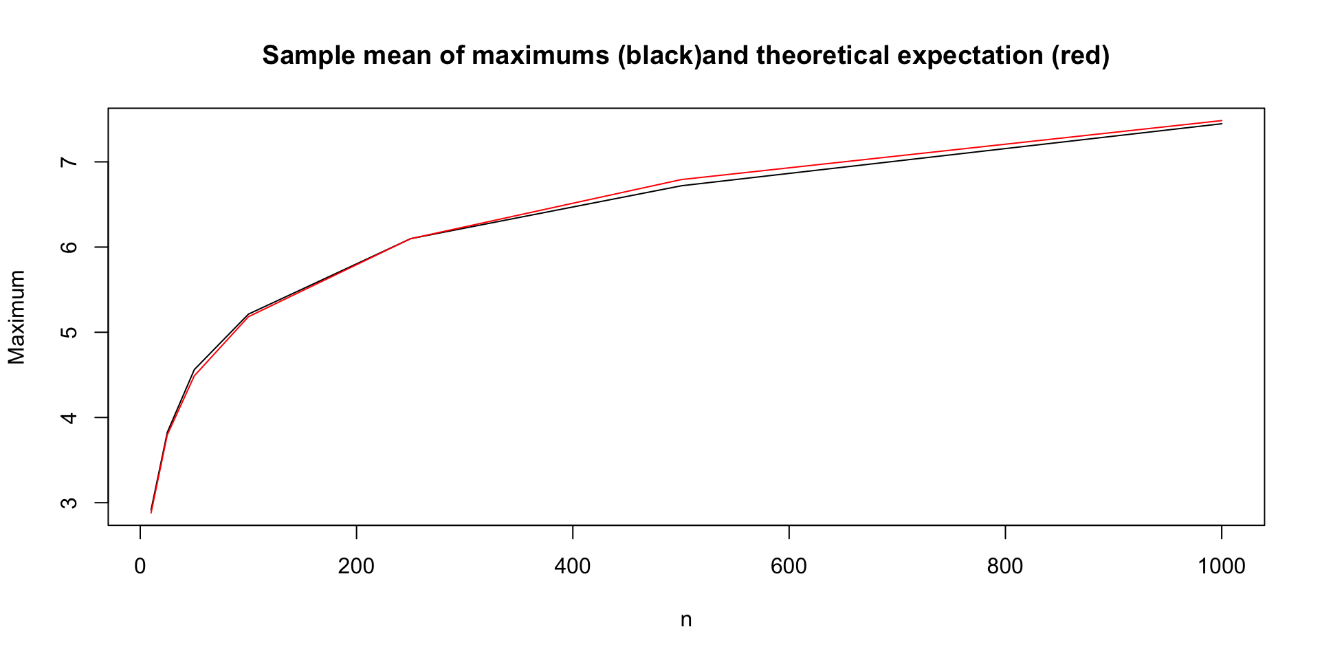
It turns out that \(\mathrm{max}(X_1,\ldots, X_n)\) can be modeled using a Gumbel distribution (after being transformed). Below, we plot the empirical mean and approximate the theoretical expectation (for large \(n\)).
Example: Maximum of random variables
