MATH167R: Simulation based inference
Overview of today
- Sampling distributions
- Bootstrap distributions
Sampling distributions
Without explicitly saying so, we have been simulating sampling distributions during our simulations.
Recall: A sampling distribution is the probability distribution of a sample-based statistic.
Example: If \(X_1,\ldots, X_{100}\) are iid random variables with variance \(1\), what is the distribution of the sample mean \(\overline{X}\)?
Simulating a sampling distribution
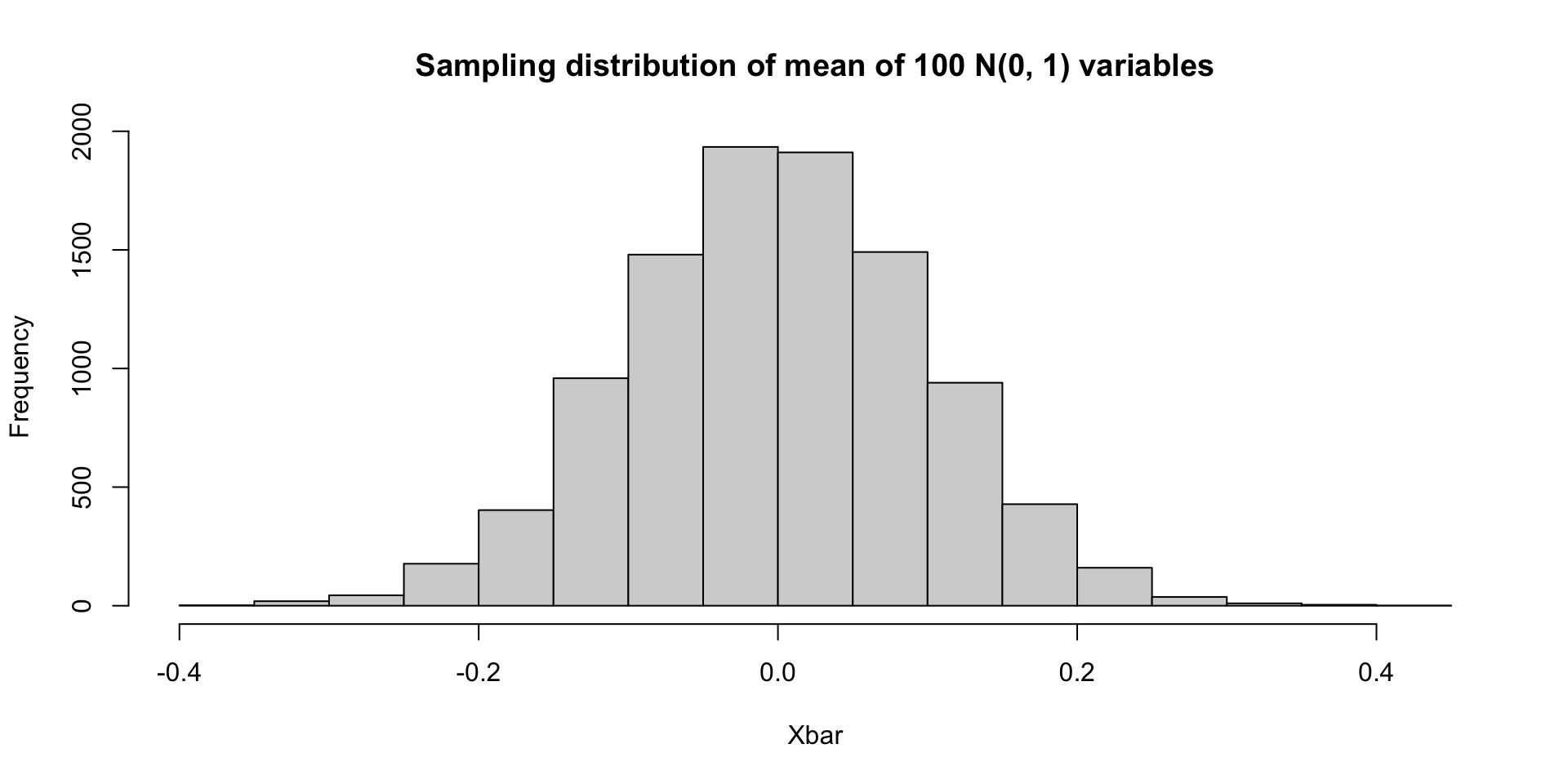
Example simulation: Suppose \(X_1,\ldots, X_{100}\sim N(0,1)\).
Simulating a sampling distribution
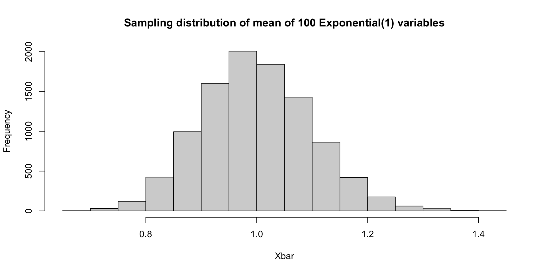
What if \(X_1,\ldots, X_{100}\sim \mathrm{Exp}(1)\)?
Simulating a sampling distribution
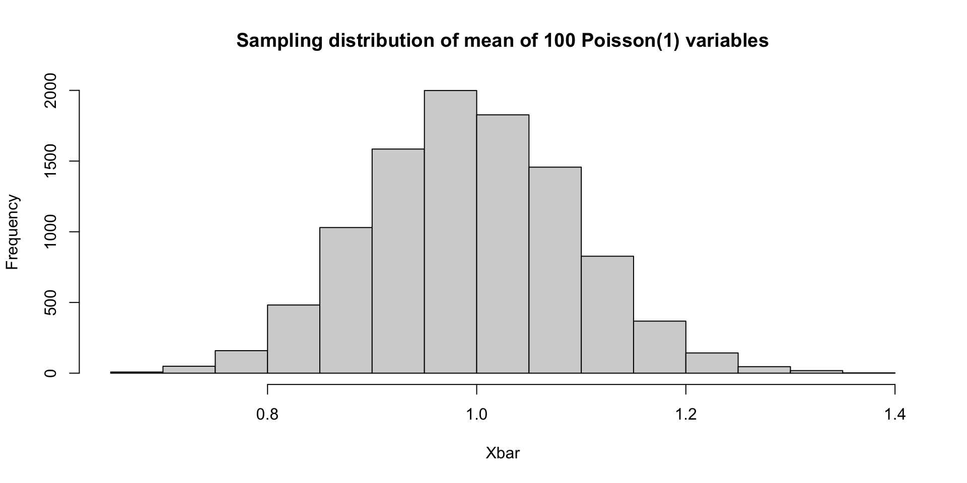
What if \(X_1,\ldots, X_{100}\sim \mathrm{Poisson}(1)\)?
Simulating a sampling distribution
By the central limit theorem, all of these sampling distributions are asymptotically Gaussian with variance 1/100 (though the mean values differ between the three). Since \(n=100\) is fairly large (for these examples), all of the previous examples are close to Gaussian.
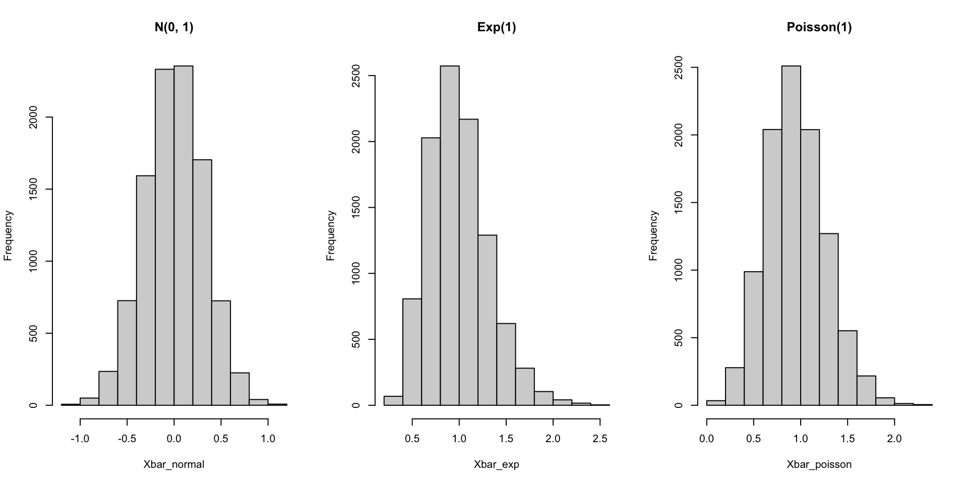
What about if \(n\) is smaller? Or if we consider other distributions?
Simulation is a powerful strategy for testing out methods:
- Suppose you wish to know… is \(n\) large?
- Create a simulation that generates data that looks like your real world data.
- Evaluate whether the results are reasonable/accurate using simulated data.
Smaller sample sizes
set.seed(123)
Xbar_normal <- replicate(10000, mean(rnorm(10)))
Xbar_exp <- replicate(10000, mean(rexp(10, rate = 1)))
Xbar_poisson <- replicate(10000, mean(rpois(10, lambda = 1)))
par(mfrow = c(1, 3))
hist(Xbar_normal, main = "N(0, 1)")
hist(Xbar_exp, main = "Exp(1)")
hist(Xbar_poisson, main = "Poisson(1)")
Smaller sample sizes
Other statistics
What if we want the sampling distribution of the maximum? For each of these population models, the sampling distribution of the maximum is different.
set.seed(123)
Xmax_normal <- replicate(10000, max(rnorm(10)))
Xmax_exp <- replicate(10000, max(rexp(10, rate = 1)))
Xmax_poisson <- replicate(10000, max(rpois(10, lambda = 1)))
par(mfrow = c(1, 3))
hist(Xmax_normal, main = "N(0, 1)")
hist(Xmax_exp, main = "Exp(1)")
hist(Xmax_poisson, main = "Poisson(1)")
Other statistics
What if we want the sampling distribution of the maximum? For each of these population models, the sampling distribution of the maximum is different.

Transformations
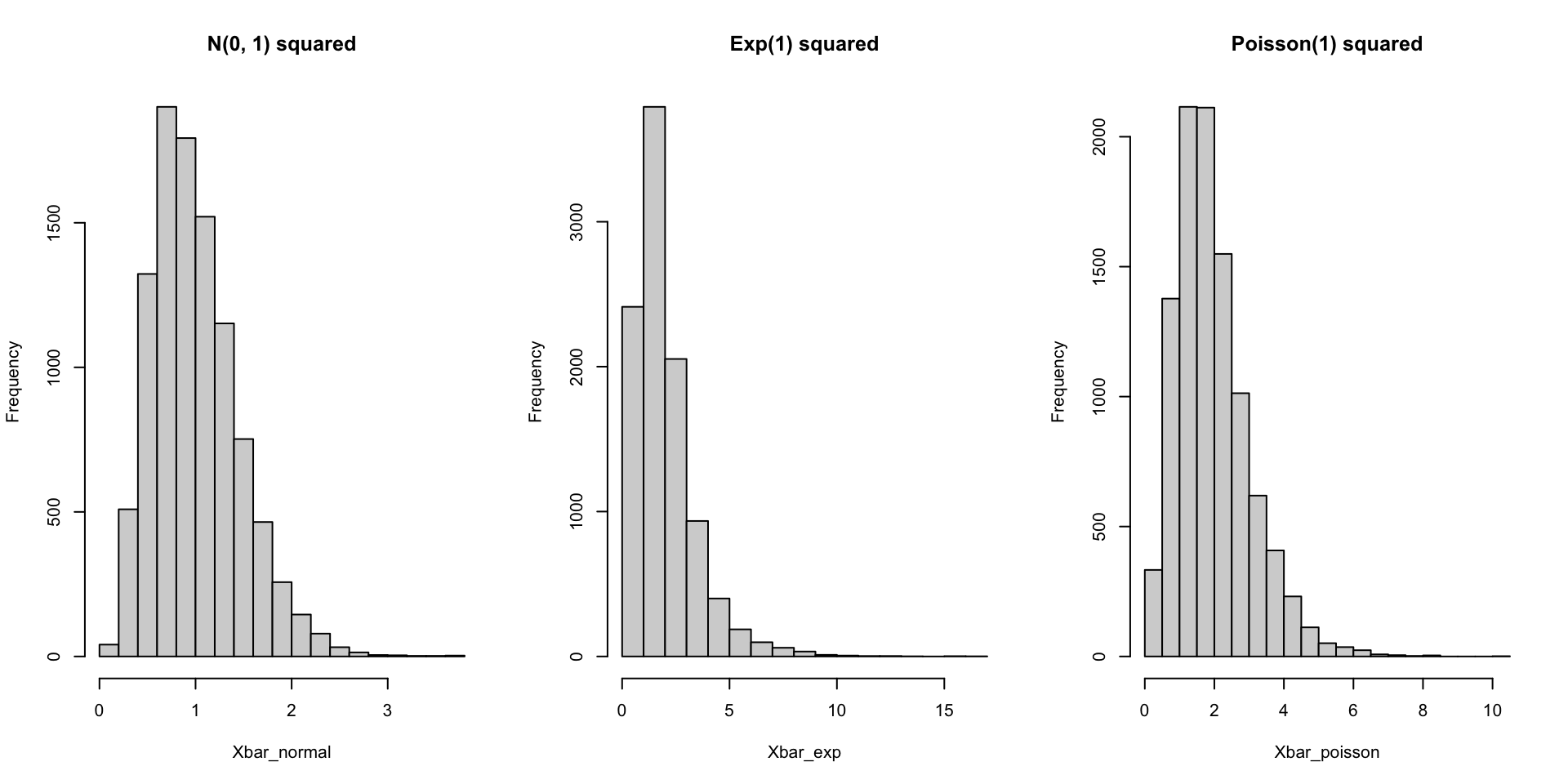
We can easily simulate sampling distributions for statistics summarizing the distribution of random variables that are defined as transformations of other random variables.
set.seed(123)
Xbar_normal <- replicate(10000, mean(rnorm(10) ^ 2))
Xbar_exp <- replicate(10000, mean(rexp(10, rate = 1) ^ 2))
Xbar_poisson <- replicate(10000, mean(rpois(10, lambda = 1) ^ 2))
par(mfrow = c(1, 3))
hist(Xbar_normal, main = "N(0, 1) squared")
hist(Xbar_exp, main = "Exp(1) squared")
hist(Xbar_poisson, main = "Poisson(1) squared")
Transformations
We can easily simulate sampling distributions for statistics summarizing the distribution of random variables that are defined as transformations of other random variables.
Exercise
- Write code to create a histogram of the sampling distribution of the sample mean \(\overline{Y}\) of \(Y_1,\ldots, Y_{10}\) where \(Y_i=\sin(X_i)\) and \(X_1,\ldots, X_{10}\) are iid Uniform(0, 1) random variables.
Resampling methods
The previous simulations are all based on parametric models (normal, exponential, Poisson). However, we can also simulate sampling distributions without parametric assumptions on the data generating mechanism.
Estimating the age of US pennies
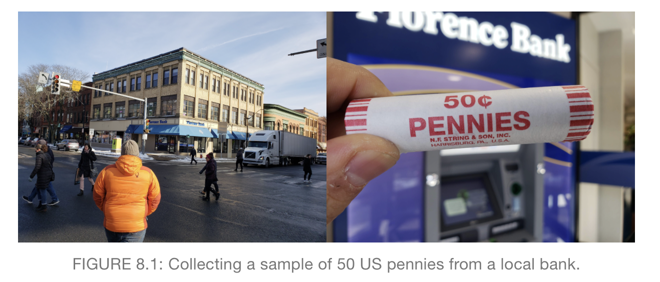
Suppose we want to estimate the average age of US pennies. We can’t observe every single penny—so what if we take a sample of 50 pennies?
Based on an example from ModernDive.
Estimating the age of US pennies
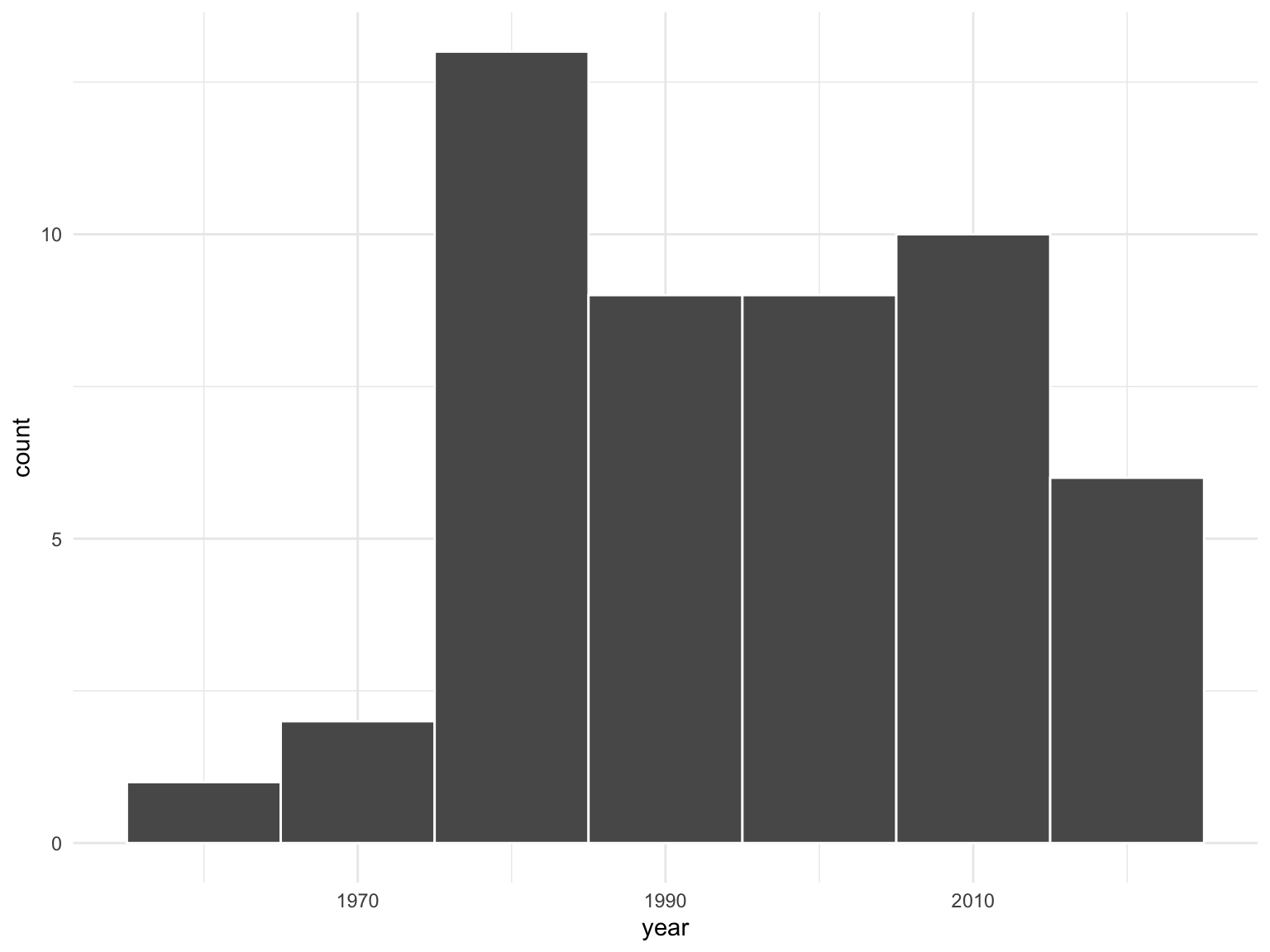
The moderndive package contains data on a sample of 50 pennies in the pennies_sample data frame.
Estimating the age of US pennies
The moderndive package contains data on a sample of 50 pennies in the pennies_sample data frame.
Estimating the age of US pennies
Based on this sample, we can compute the sample mean:
Resampling the pennies
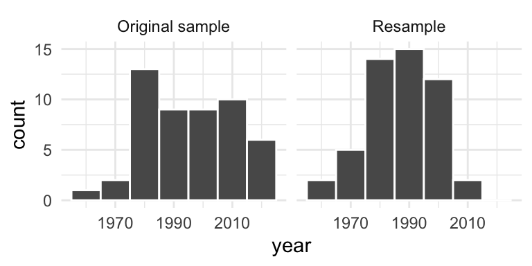
Imagine we put our 50 pennies in a bag and draw a new sample of 50 pennies by sampling with replacement. This is called resampling with replacement.
Resampling the pennies
Imagine we put our 50 pennies in a bag and draw a new sample of 50 pennies by sampling with replacement. This is called resampling with replacement.
Resampling the pennies
Note that our resample is not the same as drawing a new sample from the population. However, we can still learn about the sampling variability of the sample mean. Suppose we repeat this process many times.
Resampling the pennies
We can compute each resample mean:
Resampling the pennies
We can compute each resample mean:
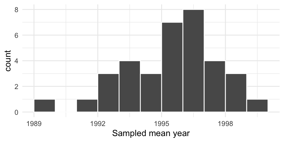
Resampling the pennies 1000 times
Using simulation, we can repeat this process virtually 1000 times:
Resampling the pennies 1000 times
Using simulation, we can repeat this process virtually 1000 times:
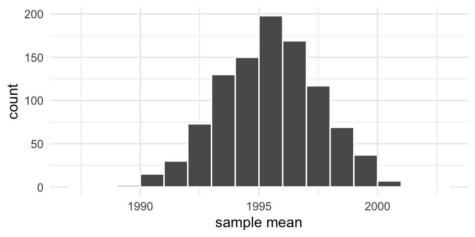
Resampling the pennies 1000 times
Note that our resampled means are centered around our original sample mean. This means that resampling doesn’t tell us about how far off our particular sample is–only about the variability of the observed values.
Resampling confidence intervals
We can obtain a confidence interval based on our resample means:
    2.5%    97.5%
1991.358 1999.441 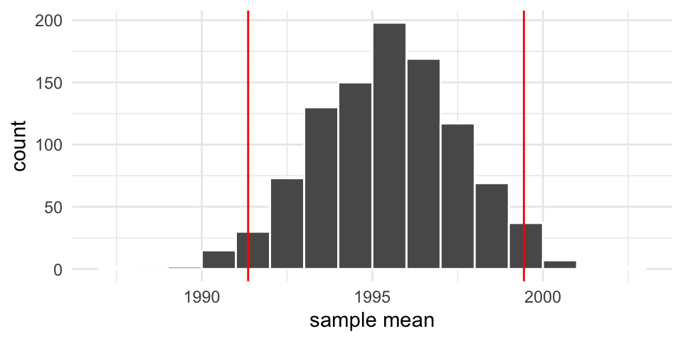
Resampling confidence intervals
Compare with a normal sampling distribution based confidence interval:
Resampling methods
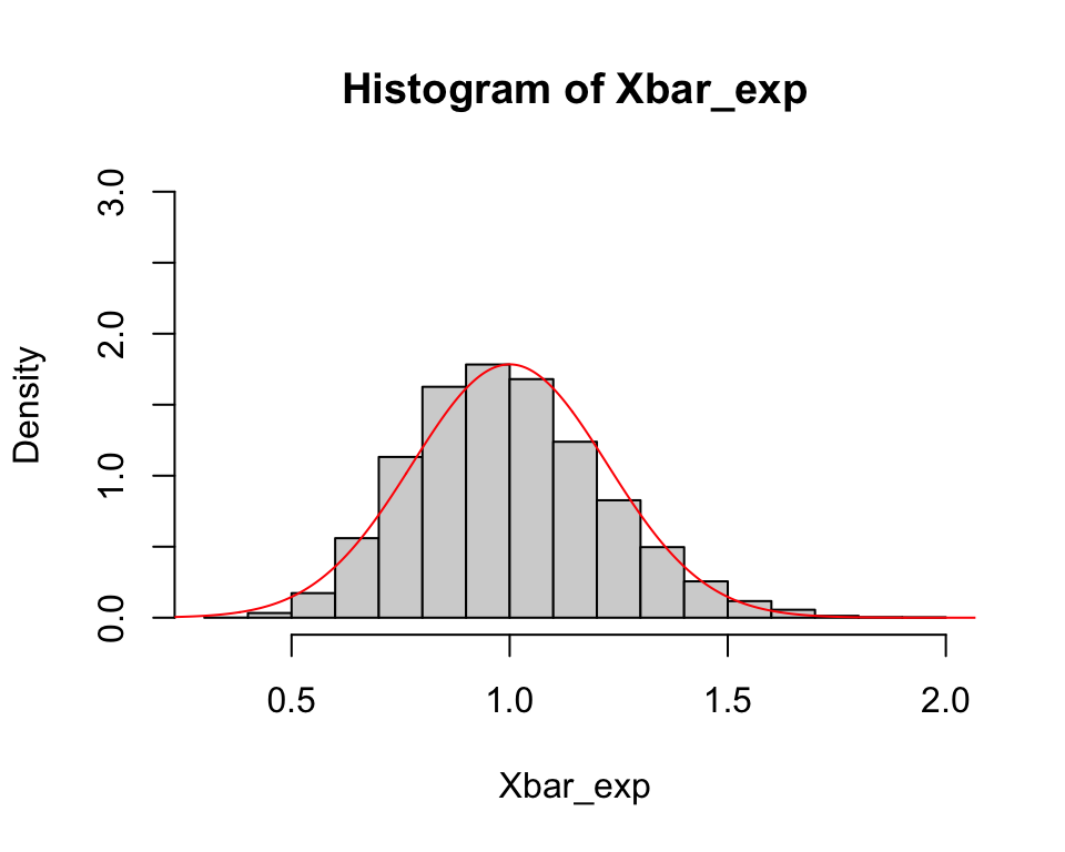
Suppose we know \(X_1,\ldots, X_{20}\sim \mathrm{Exp}(1)\). The sampling distribution of the sample mean can be simulated as follows:

Resampling methods
What if we observe \(X_1,\ldots, X_{20}\), but we don’t know that \(X_i\) is exponentially distributed? We could just try the normal approximation to approximate the sampling distribution.
Resampling methods
Bootstrap samples
Bootstrapping is a resampling method that uses random samples with replacement from the sample data to approximate the sampling distribution of sample-based statistics.
 [1] 0.00816693 0.06263315 0.11949335 0.12600941 0.14474580 0.14660666
 [7] 0.15582213 0.17485277 0.23514296 0.35492087 0.48980207 0.52215538
[13] 0.72200938 1.27034542 1.56551624 1.74866229 1.82459209 1.84311722
[19] 2.14225230 2.24995288
# sample with replacement from X
X_resample <- sample(X, size = 20, replace = TRUE)
print(sort(X_resample)) [1] 0.06263315 0.11949335 0.11949335 0.11949335 0.11949335 0.12600941
[7] 0.14474580 0.14474580 0.15582213 0.15582213 0.17485277 0.35492087
[13] 0.35492087 0.48980207 0.72200938 0.72200938 1.56551624 2.14225230
[19] 2.24995288 2.24995288Bootstrap samples
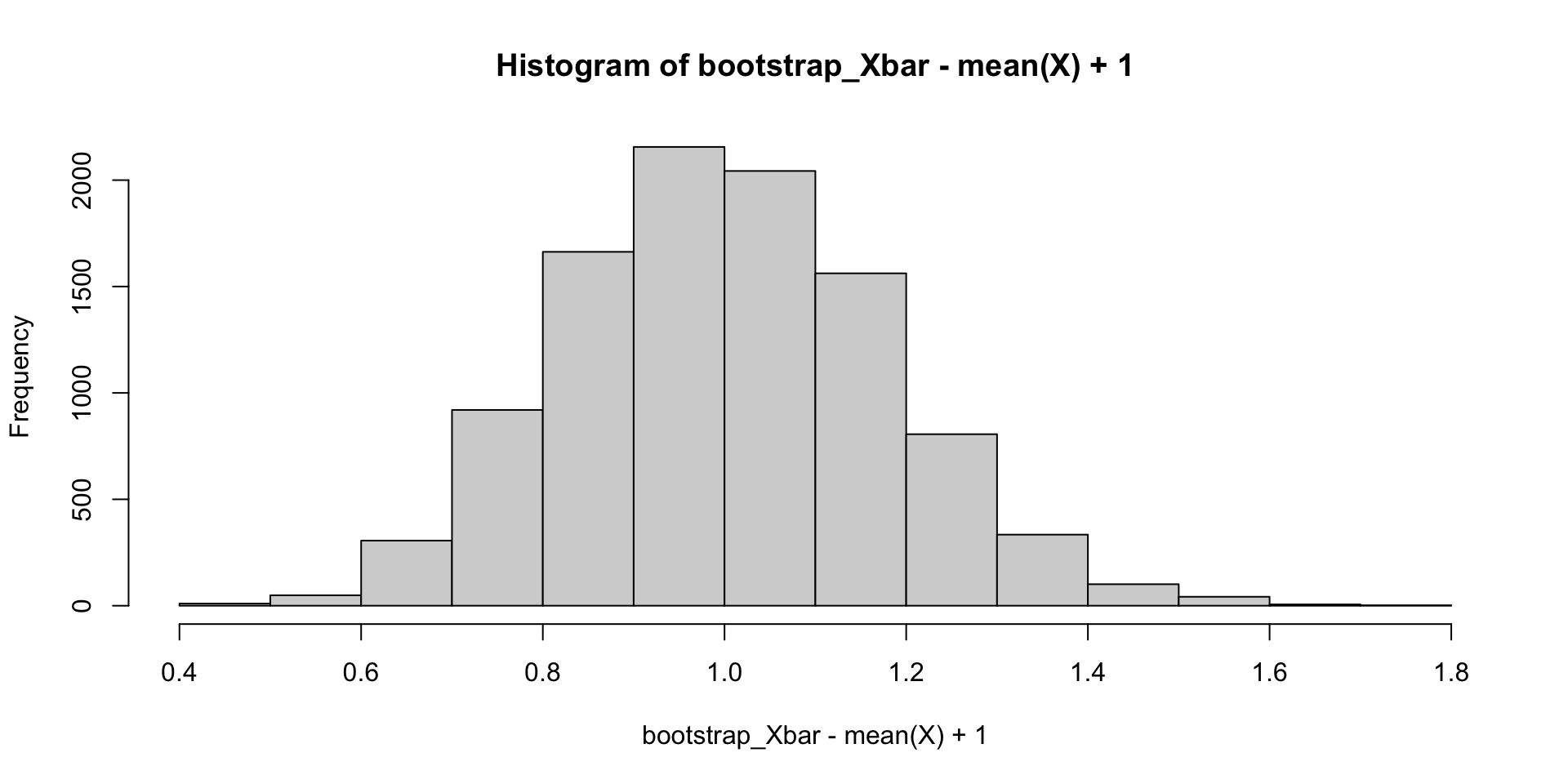
We can repeatedly resample from \(X\), then compute the resample sample means and plot the distribution:
Bootstrap samples
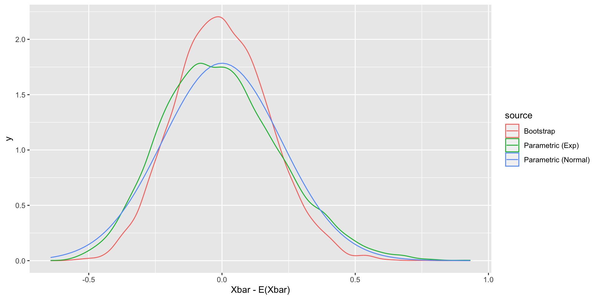
We can compare the bootstrap sampling distributions and true sampling distributions for \(\overline{X}-E(\overline{X})\).
library(ggplot2)
plot_dat <-
  data.frame(Xbar = c(Xbar_exp - 1, bootstrap_Xbar - mean(X)),
             source = rep(c("Parametric (Exp)", "Bootstrap"), each = 10000))
ggplot(plot_dat, aes(x = Xbar, color = source)) +
  geom_density() +
  geom_function(fun = dnorm,
                args = list(mean = 0, sd = 1 / sqrt(20)),
                aes(color = "Parametric (Normal)")) +
  xlab("Xbar - E(Xbar)")
Bootstrap samples
We can compare the bootstrap sampling distributions and true sampling distributions for \(\overline{X}-E(\overline{X})\).
Bootstrap confidence intervals
We can take appropriate quantiles of the bootstrap samples to construct a bootstrap confidence interval using the quantile() function:
Why bootstrap?
In this case, inference based on bootstrapping does not seem better than the normal approximation based on the central limit theorem.
However, for many cases, we may not have a simple parametric approximation to the true sampling distribution. For example, suppose we wish to compute the sampling distribution of the sample median.
Note however that the bootstrap may not work well for all statistics, such as the minimum (why not?).