MATH167R: Statistical inference

Peter Gao

Overview of today

Review of law of large numbers
Review of central limit theorem
Review of confidence intervals
Computing confidence intervals in R
Simulations with confidence intervals

Law of large numbers

We have been using simulations to estimate \(E(Y)\) where \(Y\) is some random variable. Why does this work?

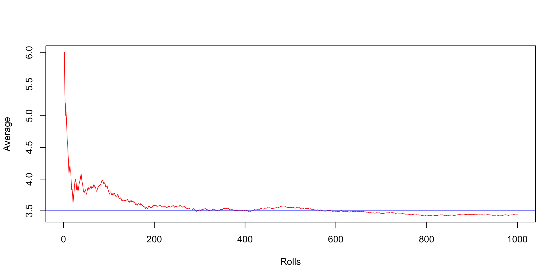
Review: The law of large numbers, informally speaking, states that if we perform the same experiment many times, the average of the observed results will be close to the expected value (and will get closer as we increase the number of trials).

The LLN can be formalized as follows: if \(X_1,\ldots, X_n\) are iid random variables with expected value \(\mu\), then the sample mean \(\overline{X}_n\) will converge to \(\mu\) (in probability or almost surely).

Law of large numbers simulation

set.seed(1028)
dice_rolls <- sample(1:6, 1000, replace = TRUE)
sample_avg <- sapply(1:length(dice_rolls), function(i) mean(dice_rolls[1:i]))
plot(1:1000, sample_avg, type = "l", col = "red",
     xlab = "Rolls", ylab = "Average")
abline(h = 3.5, col = "blue")

Central limit theorem

What does the central limit theorem say?

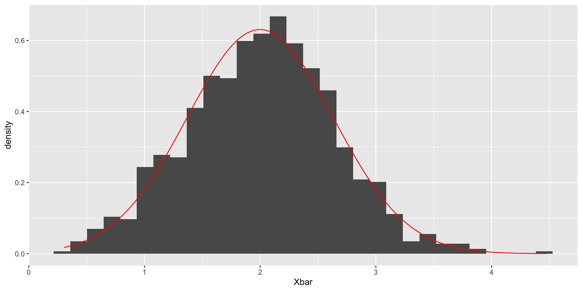
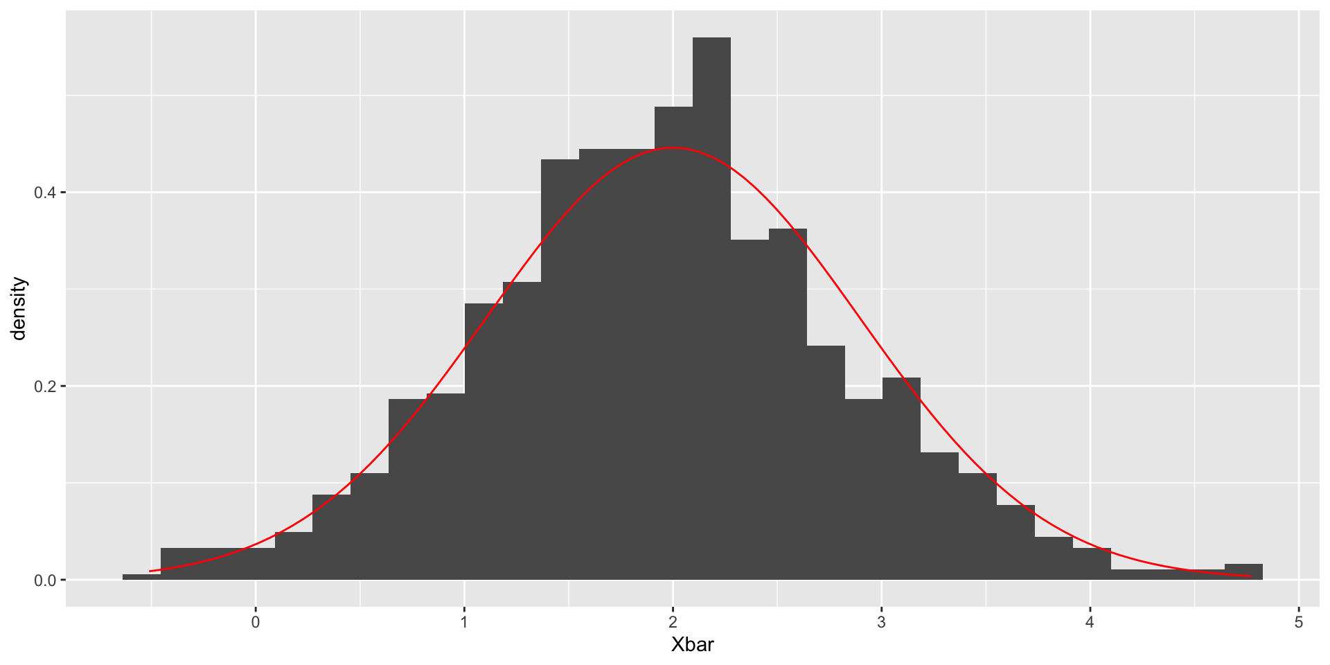
Let \(X_1,\ldots, X_n\) be independent samples from a distribution with mean \(\mu\) and variance \(\sigma^2\). Then if \(n\) is sufficiently large, \(\overline{X}_n\) has approximately a normal distribution with

\(E(\overline{X}_n)=\mu\)
\(\mathrm{Var}(\overline{X}_n)=\sigma^2/n\).

The larger the value of \(n\), the better the approximation. (Devore p. 232).

Central limit theorem

Suppose \(X_1,\ldots, X_{10}\sim N(2, 4)\):

library(ggplot2)
Xbars <- data.frame(Xbar = replicate(1000, mean(rnorm(10, mean = 2, sd = 2))))
ggplot(Xbars, aes(x = Xbar)) + 
  geom_histogram(aes(y = ..density..)) + 
  geom_function(fun = dnorm, args = list(mean = 2, sd = 2 / sqrt(10)), color = "red")

Central limit theorem

What if \(n = 5\)?

n <- 5
Xbars <- data.frame(Xbar = replicate(1000, mean(rnorm(n, mean = 2, sd = 2))))
ggplot(Xbars, aes(x = Xbar)) + 
  geom_histogram(aes(y = ..density..)) + 
  geom_function(fun = dnorm, args = list(mean = 2, sd = 2 / sqrt(n)), color = "red")

Central limit theorem

What if \(n = 5\), but \(X_1,\ldots, X_{5}\sim \mathrm{Exp}(1)\):

n <- 5
Xbars <- data.frame(Xbar = replicate(1000, mean(rexp(n, rate = 1))))
ggplot(Xbars, aes(x = Xbar)) + 
  geom_histogram(aes(y = ..density..)) + 
  geom_function(fun = dnorm, args = list(mean = 1, sd = 1 / sqrt(n)), color = "red")

Exercise

How can you break the central limit theorem?

Let \(X_1,\ldots, X_n\) be a random sample from a distribution with mean \(\mu\) and variance \(\sigma^2\). Then if \(n\) is sufficiently large, \(\overline{X}_n\) has approximately a normal distribution with \(E(\overline{X}_n)=\mu\) and \(\mathrm{Var}(\overline{X}_n)=\sigma^2/n\). The larger the value of \(n\), the better the approximation. (Devore p. 232).

What assumptions can you break?

Confidence intervals

Last class, we talked about bootstrap confidence intervals, but today we will return to the classic statistical theory for constructing confidence intervals.

A simple example: Normal population

A simple case is for constructing confidence intervals for a normally distributed population variable. If we assume

The population distribution is normal
The value of the population standard deviation \(\sigma\) is known

Given samples \(X_1,\ldots, X_n\), we can compute \(\overline{X}_n\) and then

\[\frac{\overline{X}_n-\mu}{\sigma/\sqrt{n}}\sim N(0, 1)\]

A simple example: Normal population

We can thus compute a 95% confidence interval:

\[P\left(-1.96< \frac{\overline{X}_n-\mu}{\sigma/\sqrt{n}}<1.96\right)=.95\]

Algebraic manipulation yields

\[P\left(\overline{X}_n-1.96\frac{\sigma}{\sqrt{n}}<\mu<\overline{X}_n+1.96\frac{\sigma}{\sqrt{n}}\right)=.95\]

The final interval can be written as \(\overline{X}_n\pm 1.96(\sigma/\sqrt{n})\).

A simple example: Normal population

In general, for a \(100(1-\alpha)\%\) confidence interval, we can use

\[P\left(-z_{\alpha/2}< \frac{\overline{X}_n-\mu}{\sigma/\sqrt{n}}<z_{\alpha/2}\right)=1-\alpha\]

where \(z_{\alpha/2}\) is defined by \(1 - P(Z\leq z_{\alpha/2})=\alpha/2\). This yields the interval

\[\overline{X}_n\pm z_{\alpha/2}(\sigma/\sqrt{n})\]

Interpretation

Consider the equation

\[P\left(\overline{X}_n-1.96\frac{\sigma}{\sqrt{n}}<\mu<\overline{X}_n+1.96\frac{\sigma}{\sqrt{n}}\right)=.95\]

Which elements of this equation are random?

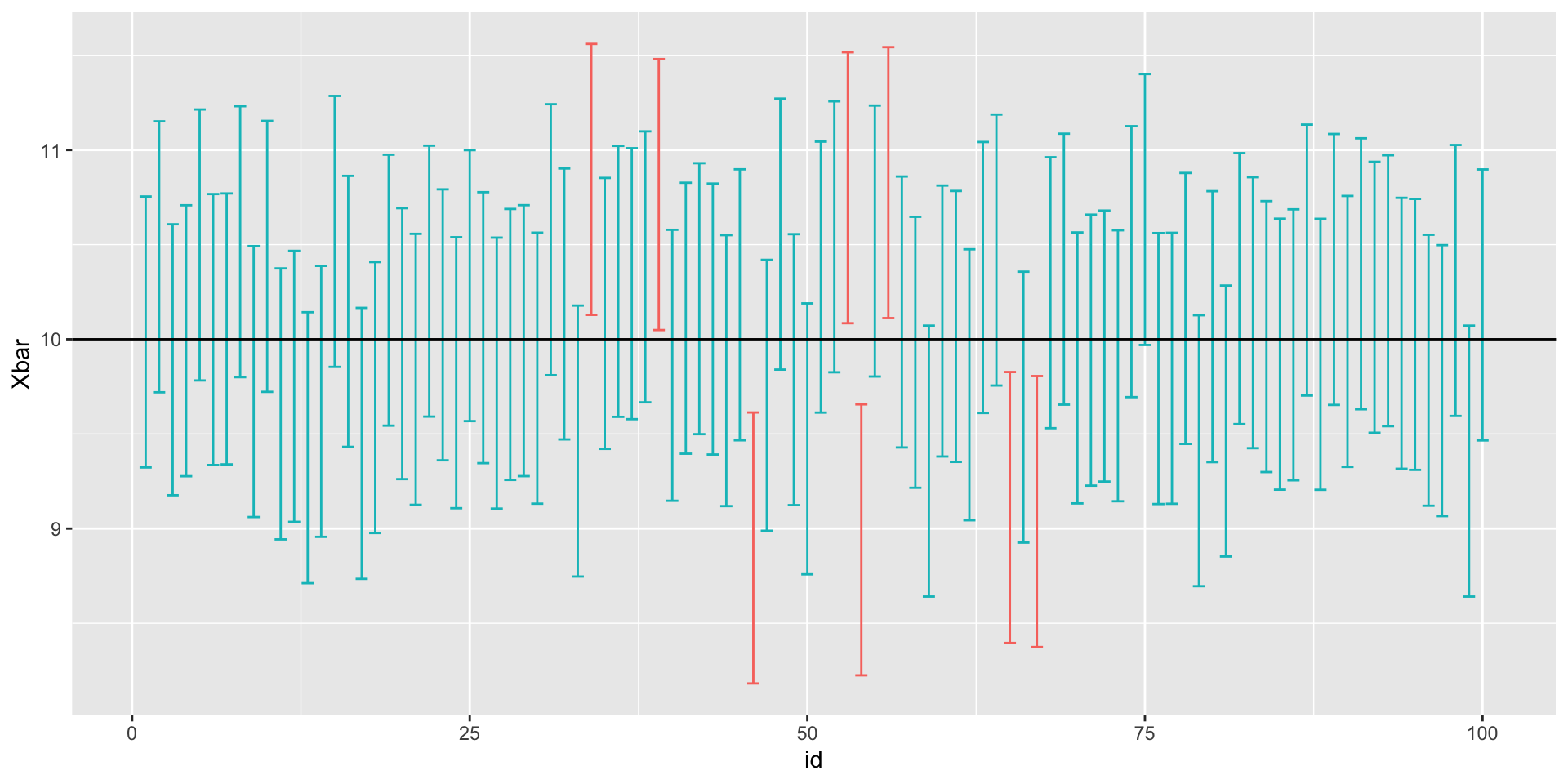
Remember, \(\overline{X}_n\) and thus the interval itself are random. Prior to observing the data and computing \(\overline{X}_n\), there is a .95 probability that the interval will include the true value of \(\mu\).

However, we cannot say anything about the probability that any particular confidence interval contains \(\mu\).

Example (Devore 7.1)

A sample of \(n=31\) trained typists was selected, and the preferred keyboard height was determined for each typist. The resulting sample average preferred height was \(x=80.0\)cm.

Assuming that the preferred height is normally distributed with \(\sigma = 2.0\)cm, obtain a 95% confidence interval (interval of plausible values) for \(\mu\), the true average preferred height.

\[\overline{X}_n\pm 1.96\frac{2.0}{\sqrt{31}}=80.0\pm .7=(79.3, 80.7)\]

Simulating many confidence intervals

n <- 30 # sample size
mu <- 10 # unknown true mean
sigma <- 2 # known standard deviation
Xbars <- replicate(100, mean(rnorm(n, mean = mu, sd = sigma)))
coverage_rate <- mean(abs(Xbars - mu) < 1.96 * sigma / sqrt(n))
coverage_rate

[1] 0.92

Simulating many confidence intervals

Code to visualize all of our confidence intervals:

library(tidyverse)
plot_dat <- data.frame(id = 1:100,
                       Xbar = Xbars) |>
  mutate(upper = Xbar + 1.96 * sigma / sqrt(n),
         lower = Xbar - 1.96 * sigma / sqrt(n))
ggplot(plot_dat, 
       aes(x = id, y = Xbar, 
           color = abs(Xbars - mu) < 1.96 * sigma / sqrt(n))) + 
  geom_errorbar(aes(ymin = lower, ymax = upper)) +
  geom_abline(intercept = mu, slope = 0) + 
  theme(legend.position = "none")

Simulating many confidence intervals

Large-sample confidence intervals

What if we do not know whether the population distribution is normal? Provided \(n\) is sufficiently large, the CLT implies that \(\overline{X}_n\) is approximately normal regardless of the population distribution.

What if we do not know \(\sigma?\) Again, provided \(n\) is sufficiently large, we can replace \(\sigma\) with the sample standard deviation \(S\).

We obtain the confidence interval formula:

\[\overline{X}_n\pm z_{\alpha/2}(S/\sqrt{n})\]

Simulating many confidence intervals

n <- 30 # sample size
lambda <- 10
sample_stats_poisson <- function() {
  x <- rpois(n, lambda)
  return(c(mean(x), sd(x)))
}
stats <- replicate(100, sample_stats_poisson())
stats[, 1:5] # print out first five simulation results

          [,1]      [,2]      [,3]     [,4]     [,5]
[1,] 10.666667 10.733333 10.500000 9.633333 9.800000
[2,]  2.940013  2.702915  2.933164 2.953471 3.252585

coverage_rate <- mean(abs(stats[1,] - mu) < 1.96 * stats[2,] / sqrt(n))
coverage_rate

[1] 0.98

When \(n\) is small but \(\sigma\) unknown: \(t\)-intervals

What about when \(n\) is small, but \(\sigma\) is unknown? Assuming again that the population distribution is normal,

\[T=\frac{\overline{X}_n-\mu}{S/\sqrt{n}}\]

has a \(t\) distribution with \(n-1\) degrees of freedom. We can thus use the confidence interval

\[\overline{X}_n\pm t_{\alpha/2, n-1}(S/\sqrt{n})\] where \(P(T\leq t_{p, n-1})=p\) when \(T\) follows a \(t\)-distribution with \(n-1\) degrees of freedom.

Assessing normality of the population distribution

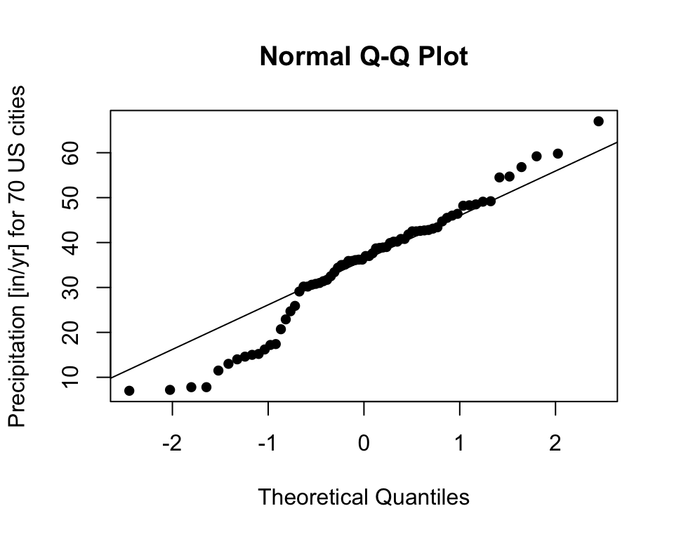
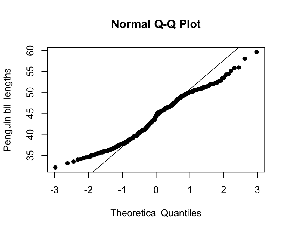
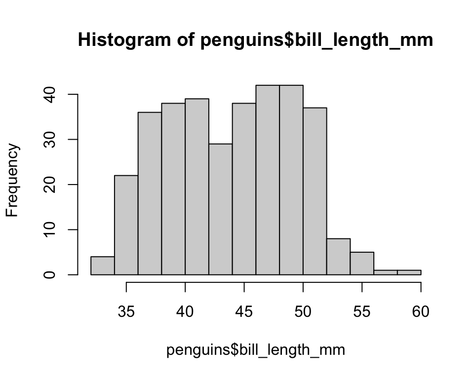
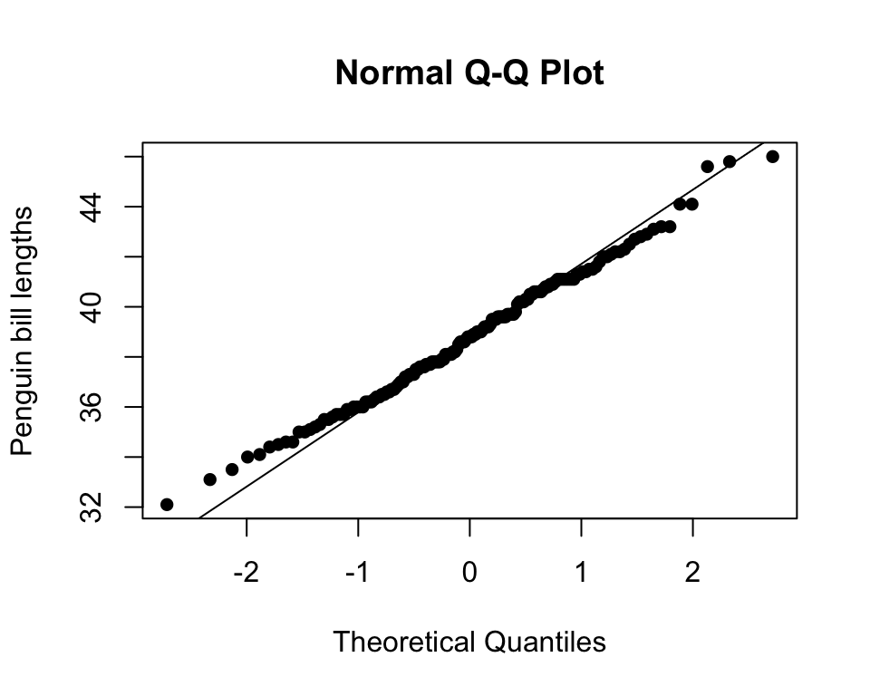
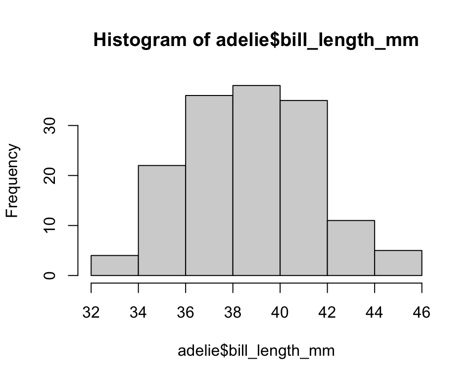
How can we tell if the population distribution is normal? One simple check is to use a quantile-quantile (QQ) plot.

Using your data, estimate the quantiles using the empirical distribution.
Compare the sample quantiles with the quantiles of a known distribution (often normal).
If the sample and theoretical quantiles appear to fall on a line, then the empirical distribution function will be similar to (a scaled version of) the theoretical distribution function.

Example: Precipitation

The precip dataset includes annual precipitation in inches for a number of US cities. Is this normally distributed?

head(precip)

     Mobile      Juneau     Phoenix Little Rock Los Angeles  Sacramento 
       67.0        54.7         7.0        48.5        14.0        17.2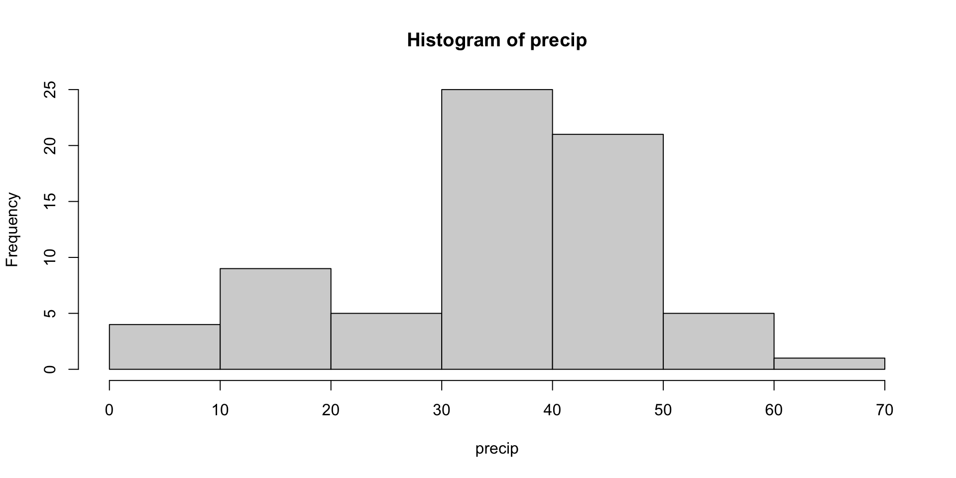

hist(precip)

Example: Precipitation

The qqnorm() function can be used to compare the empirical/sample quantiles and the theoretical quantiles of a standard normal. The qqline() function adds a line that passes through the first and third quartiles.

qqnorm(precip, ylab = "Precipitation [in/yr] for 70 US cities", pch = 16)
qqline(precip)

Example: Penguins

library(palmerpenguins)
data(penguins)
qqnorm(penguins$bill_length_mm, ylab = "Penguin bill lengths", pch = 16)
qqline(penguins$bill_length_mm)

Example: Penguins

hist(penguins$bill_length_mm)

Example: Penguins

adelie <- penguins |> dplyr::filter(species == "Adelie")
qqnorm(adelie$bill_length_mm, ylab = "Penguin bill lengths", pch = 16)
qqline(adelie$bill_length_mm)

Example: Penguins

hist(adelie$bill_length_mm)

Using R to compute confidence intervals

Generally, if you are only doing a simple normal-based or \(t\)-based confidence interval for a mean, I recommend computing \(\overline{X}_n\) and \(S\) using mean() and sd(), and then computing the confidence interval by hand.

You can also use the t.test() function to compute the appropriate \(t\)-interval for a population mean:

precip_t <- t.test(precip, conf.level = 0.95)
precip_ci <- precip_t$conf.int # get confidence interval
precip_ci

[1] 31.61748 38.15395
attr(,"conf.level")
[1] 0.95

Comparing \(t\)-based and bootstrap confidence intervals

bootstrap_Xbar <- 
  replicate(10000, mean(sample(precip, size = length(precip), replace = TRUE)))
quantile(bootstrap_Xbar, probs = c(.025, .975))

    2.5%    97.5% 
31.78282 38.07286

precip_ci

[1] 31.61748 38.15395
attr(,"conf.level")
[1] 0.95

In this case, since \(n\) is large, the non-normality is not a big deal.

Confidence intervals for proportions

For large \(n\), the following confidence interval is often used for a population proportion:

\[\widehat{p}\pm z_{\alpha/2}\sqrt{\frac{\widehat{p}(1-\widehat{p})}{n}}\]

Note that this formula only gives an approximate CI because of the use of \(\widehat{p}\) when estimating the standard error of \(\widehat{p}\).

Other confidence intervals

R has implementations for confidence intervals for many types of population parameters, including for non-normally distributed populations. Always carefully read the documentation before using these functions.