set.seed(302)
# the true population parameter (in practice, we don't know this).
p <- 0.6
# simulate 100 coin flips
coin_flips <- rbinom(100, size = 1, prob = p)
head(coin_flips)
[1] 1 0 0 1 1 1[1] 61Hypothesis testing always begins with a scientific question of interest. Suppose we have a coin, and we want to test whether or not it is fair. We might flip the coin over and over and record the results, and then measure the proportion of times we got a heads.
We can state this experiment more formally. Let \(X_1,...,X_n\) be \(n\) random variables corresponding to an indicator of whether a coin flip is heads (i.e. \(X_i = 1\) if the \(i\)th flip is heads, \(0\) if tails). We don’t know the true probability that our coin lands on heads, so we may say that \[X_i \stackrel{iid}{\sim} \mathrm{Binomial}(1, p),\] with unknown probability parameter \(p\).
We are interested in whether our coin is fair, which corresponds to \(p=1/2\). This hypothesis we are interested in testing will be our null hypothesis, denoted \(H_0\) (pronounced “H-naught” or “H-zero”).
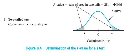
Alternatively, we may think that our coin is biased in either direction (i.e. either lands on heads too often or lands on tails too often). This corresponds to \(p \neq 1/2\). This is our alternative hypothesis, denoted \(H_a\) (or sometimes \(H_1\)).
Thus, our hypothesis test is as follows:
\[\begin{align} H_0: p&=1/2\\ H_a: p&\neq 1/2 \end{align}\]In general, we can think of
Null hypothesis \(H_0\): our default assumption to be tested, our baseline, no relationships/differences/values of our parameters of interest. Assumed to be true unless evidence suggests otherwise!
Alternative hypothesis \(H_a\): the alternative to our null, something interesting is happening in our data, our scientific hypothesis of interest
An important note: for the most part, these are broad generalizations, not formal definitions.
It is not always the case that the alternative is “interesting” and the null is not.
We always assume that our null hypothesis is true to compute the null distribution.
Our question is whether our data provides sufficient evidence to reject the null \(H_0\).
For example, if we flipped our coin 100 times and observed 99 heads, we probably would reject our null hypothesis that the coin is fair. If instead we flipped our coin 100 times and observed 52 heads, we probably would not conclude that we have enough evidence to reject our null hypothesis, and maintain our baseline assumption that the coin is fair.
Where we assume something is true, and then observe whether or not the evidence (data) supports this assumption.
In hypothesis testing, we never, ever, ever examine whether our evidence supports our scientific hypothesis (the alternative). We only examine whether it supports rejecting a baseline assumption (the null).
Statistical inference: using information from a sample to draw inferences about a population.
Usually we are interested in studying/estimating a population parameter: a numerical characteristic of our population/model.
Example of a model/population: an infinite sequence of coin flips distributed \(Bin(1, p)\).
Example of a parameter: the probability of heads \(p\).
We use estimators to calculate estimates for our parameters.
Estimator: a function of our data (for example, the sample mean)
Estimate: the actually observed value of our estimator, anumber calculated from our data (for example, an observed sample mean of 52).
Back to our example, recall that we aim to test
\[\begin{align} H_0: p&=1/2\\ H_a: p&\neq 1/2 \end{align}\]using a random variable representing a heads \[X_i \stackrel{iid}{\sim} Bin(1, p).\] Let’s assume that we have the patience to flip our coin \(n=100\) times.
Instead of actually flipping the coin, let’s carry out this example in R.
set.seed(302)
# the true population parameter (in practice, we don't know this).
p <- 0.6
# simulate 100 coin flips
coin_flips <- rbinom(100, size = 1, prob = p)
head(coin_flips)[1] 1 0 0 1 1 1[1] 61We observed 61 heads out of 100 coin flips. This is our test statistic, a statistic calculated from our sample data which we will use to evaluate our hypotheses.
We observed 61 heads out of 100 coin flips.
Is this unusual enough to reject \(H_0\)?
In order to answer this, we must ask ourselves: if we assume \(H_0\) is true, how unlikely is what we observed? Before we conduct our experiment, we must decide what cut-off we would like to use to determine whether or not to reject \(H_0\). This cut-off is typically denoted by the greek letter \(\alpha\).
Typically, we reject \(H_0\) if the probability of observing a test statistic as or more extreme than what we observed is less than 5%. We will use this cut-off, even though it is arbitrary.
Thus, we set \(\alpha = 0.05\).
We can use pbinom() to calculate the probability of observing a test statistic as extreme or more extreme than 61.
Note that lower.tail = TRUE is the default, and returns the probability of observing a value less than or equal to the value that we input. Thus, when lower.tail = FALSE, we return the probability of observing a value strictly greater than the value that we input. We want the probability of observing a value greater than or equal to the value that we input. Thus, we subtract 1 to make sure this value is included in our probability.
# record test statistic
test_stat <- sum(coin_flips)
# record how "extreme" our test statistic is
diff_from_exp <- abs(50 - test_stat)
# first component: lower tail
# second component: upper tail
p_val <- pbinom(50 - diff_from_exp, size = 100, prob = 0.5) +
  pbinom(50 + diff_from_exp - 1, size = 100, prob = 0.5, lower.tail = FALSE)
round(p_val, 3)
[1] 0.035Note that lower.tail = TRUE is the default, and returns the probability of observing a value less than or equal to the value that we input. Thus, when lower.tail = FALSE, we return the probability of observing a value strictly greater than the value that we input. We want the probability of observing a value greater than or equal to the value that we input. Thus, we subtract 1 to make sure this value is included in our probability.
\(P(\text{test statistic equally or more extreme than observed}|H_0) =\) 0.035.
\(P(\text{test statistic equally or more extreme than observed}|H_0) =\) 0.035.
This is less than our pre-determined cut-off of 0.05, so we conclude that our results are statistically significant. This means that we reject \(H_0\) and have evidence to support our alternative hypothesis \(H_a\), that our coin is biased. With that conclusion, we have completed our hypothesis test.
Note that we do not conclude that \(H_0\) is false, or that \(H_a\) is true. We only state our conclusion in terms of sufficient evidence to reject the null or insufficient evidence to reject the null.
Remember, a \(P\)-value is not the probability our null hypothesis is true. A \(P\)-value only describes the probability of observing results as extreme or more extreme than our results under the null distribution.
Problems begin when our null distribution is misspecified (for example, when assumptions are broken).
(Devore)
Suppose we wish to see whether our data represents evidence for the existence of “facial stereotypes.”
t.test(): t-tests in RConducting t-tests in R is very easy using the function t.test(). For a two sample t-test to compare the means of two samples, just provide the two samples in R. Here I use randomly simulated data. This performs a test of the form:
\[ \begin{align} H_0: \mu_x &= \mu_y\\ H_a: \mu_x &\neq \mu_y \end{align} \]
t.test(): t-tests in R
    Welch Two Sample t-test

data:  x and y
t = -1.5143, df = 16.95, p-value = 0.1484
alternative hypothesis: true difference in means is not equal to 0
95 percent confidence interval:
 -1.627018  0.267543
sample estimates:
mean of x mean of y
0.3492983 1.0290359 t.test(): t-tests in RNote that we can also test one-sided hypotheses:
\[ \begin{align} H_0: \mu_x &= \mu_y\\ H_a: \mu_x &< \mu_y \end{align} \]
t.test(): t-tests in RWe can also use a one sample t-test to compare the means of one sample to some hypothesized value.
This performs a test of the form:
\[ \begin{align} H_0: \mu_x &= 0\\ H_a: \mu_x &\neq 0 \end{align} \]
t.test(): t-tests in RWhich is worse?
It probably depends on the scenario.
Type I errors are false positives–we obtain a “statistically significant” result via chance.
Note that we typically control the type I error through the significance level \(\alpha\).
\[\Large \alpha = P(\text{reject } H_0 | H_0 \textrm{ true}))\]
\[\Large 1-\alpha = P(\text{don't reject } H_0 | H_0 \textrm{ true})\]
Type 2 errors are false negatives–we incorrectly fail to reject the null hypothesis when the null hypothesis is actually false.
\[ P(\text{type 2 error}) = P(\text{fail to reject } H_0 | H_0 \text{ is false})\]
Type 2 error also gives us the concept of power, the probability of correctly rejecting the null.
\[ \text{Power} = P(\text{reject } H_0 | H_0 \text{ is false})\]
In many scientific settings, there has been an emphasis on producing results with statistically significant p-values. However, note that by repeatedly performing hypothesis tests, you are very likely to produce statistically significant results, even if the null hypothesis is true.
This has led to a crisis in replication, in which the results of many scientific studies are difficult or impossible to replicate.
P-hacking refers to the practice of repeatedly performing hypothesis tests (and potentially manipulating the data) until a statistically significant P-values is obtained. Usually, only this final result is published, without mentioning all of the manipulations that came before.
For this reason, it’s crucial to document carefully everything you do in the data analysis pipeline to ensure that your work is taken seriously. Publishing code and data can help others to reproduce your research.