MATH167R: Hypothesis Testing

Peter Gao

Overview of today

Review of basic hypothesis tests
Designing your own hypothesis test
Permutation tests

Summary: hypothesis testing

Define null and alternative hypotheses.
- ex. \(H_0:\mu = 0\) and \(H_a:\mu\neq 0\)
Compute a test statistic for which the null sampling distribution is known (based on assumptions about the population/sample).
- ex. \(T=(\overline{X}_n-\mu)/(S^2/\sqrt{n})\sim t_{n-1}\)
Compare the test statistic with the null distribution to obtain a P-value.
- ex. \(P(|T|>|t|)\) where \(t\) is the observed test statistic.

Example: Two-sample \(z\)-test

Assumptions:

\(X_1, \ldots, X_m\) is a random sample from a distribution with mean \(\mu_1\) and variance \(\sigma_1^2\).
\(Y_1, \ldots, Y_n\) is a random sample from a distribution with mean \(\mu_2\) and variance \(\sigma_2^2\).
The \(X\) and \(Y\) samples are independent of one another.
The sample sizes are adequately large (usually appropriate if \(m>40\) and \(n>40\).

Example: Two-sample \(z\)-test

Hypotheses:

H_0: \(\mu_1=\mu_2\)
H_a: \(\mu_1\not=\mu_2\)

Example: Two-sample \(z\)-test

Under these assumptions, \(\overline{X}-\overline{Y}\) is approximately normal and the test statistic \[Z=\frac{\overline{X}-\overline{Y}-(\mu_1-\mu_2)}{\sqrt{\frac{S_1^2}{m}+\frac{S_2^2}{n}}}\] has approximately a standard normal distribution when \(H_0\) is true.

Example: Two-sample \(t\)-test

When the samples are small, but the population distributions are approximately normal, the standardized test statistic \[T=\frac{\overline{X}-\overline{Y}-(\mu_1-\mu_2)}{\sqrt{\frac{S_1^2}{m}+\frac{S_2^2}{n}}}\] has approximately a \(t\) distribution with df \(v\) estimated from the data by

\[\nu =\frac{\left(\frac{s_1^2}{m}+\frac{s_2^2}{n}\right)^2}{\frac{(s_1^2/m)^2}{m-1}+\frac{(s_2^2/n)^2}{n-1}}\]

Example: Two-sample \(t\)-test

We can use the sleep data in R, which contains Student’s example data on the effect of two sleeping drugs on 10 patients, to test out the t.test() function.

t.test(extra ~ group, data = sleep)


    Welch Two Sample t-test

data:  extra by group
t = -1.8608, df = 17.776, p-value = 0.07939
alternative hypothesis: true difference in means between group 1 and group 2 is not equal to 0
95 percent confidence interval:
 -3.3654832  0.2054832
sample estimates:
mean in group 1 mean in group 2 
           0.75            2.33

“There is only one test”

Image by Allen Downey

“There is only one test”: Tim and Bob

Lea et al. (2007)

“There is only one test”: Tim and Bob

Image by Allen Downey

What is the data? Test statistic? Model of \(H_0\)? P-value?

Designing your own hypothesis test

Suppose we have five sequences of 200 coin flips.

# A tibble: 6 × 5
  A     B     C     D     E    
  <chr> <chr> <chr> <chr> <chr>
1 T     H     H     T     H    
2 H     H     H     H     H    
3 T     H     T     H     H    
4 H     T     H     H     H    
5 H     T     T     H     T    
6 T     H     T     T     H

Only one sequence is generated by flipping a fair coin, using the code sample(c("H", "T"), 200, replace = T).

Can we design a hypothesis test to help us identify the true sequence?

This activity adapted from a blog post from Alex Hayes.

Designing your own hypothesis test

First, load the flips using the following code.

library(tidyverse)
flips <- read_csv("https://math167r-s24.github.io/static/flips.csv")
head(flips)

# A tibble: 6 × 5
  A     B     C     D     E    
  <chr> <chr> <chr> <chr> <chr>
1 T     H     H     T     H    
2 H     H     H     H     H    
3 T     H     T     H     H    
4 H     T     H     H     H    
5 H     T     T     H     T    
6 T     H     T     T     H

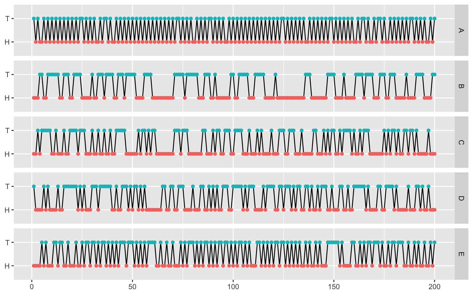
Can you tell which is real and which are fake?

Visual inspection

flips_long <- flips |>
  mutate(id = 1:200) |>
  pivot_longer(-id,  names_to = "Sequence", values_to = "Flip")

flips_long |> 
  ggplot(aes(x = id, y = Flip, group = Sequence)) +
  geom_line() +
  geom_point(aes(color = Flip)) +
  facet_grid(rows = vars(Sequence)) + 
  theme(
    legend.position = "none",
    axis.title = element_blank()
  )

A simple test: Counting the number of heads

We can use the test we discussed last class for a sample proportion:

\[\begin{align} H_0: p&=1/2\\ H_a: p&\neq 1/2 \end{align}\]

where we assume that the flips \(X_1,...,X_n\) are iid \(X_i \stackrel{iid}{\sim} \mathrm{Binomial}(1, p)\) with probability of heads \(p\).

A simple test: Counting the number of heads

What are the test statistics for each of our sequences? One option is to use the total number of heads.

# A tibble: 5 × 2
  Sequence nHeads
  <chr>     <int>
1 A           100
2 B           108
3 C           114
4 D           101
5 E            98

A simple test: Counting the number of heads

Do any of these indicate that certain sequences are fake? How could we get corresponding P-values?

Approach one: Use the normal approximation: \[\widehat{p}\sim N\left(p, \sqrt{\frac{p(1-p)}{n}}\right)\]

phats <- flips_long |>
  group_by(Sequence) |>
  summarize(phat = mean(Flip == "H"))
# two-sided p-values
(1 - pnorm(abs(phats$phat - .5), sd = sqrt(.5 * .5 / 200))) * 2

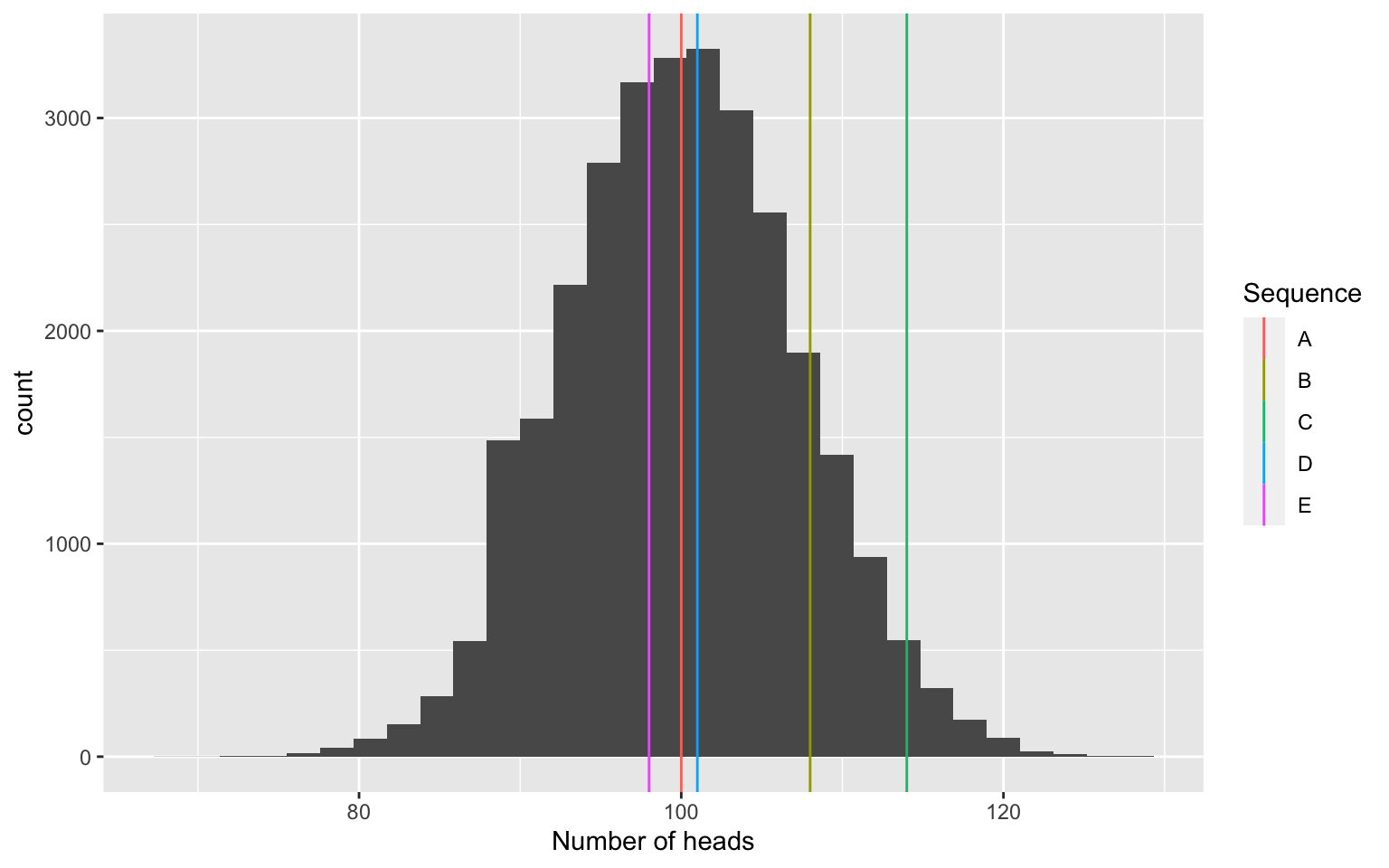
[1] 1.00000000 0.25789904 0.04771488 0.88753708 0.77729741

This suggests that sequence C has too many heads.

A simple test: Counting the number of heads

Approach two: Use simulations to estimate the distribution of number of heads under the null:

A simple test: Counting the number of heads

Approach two: Use simulations to estimate the distribution of number of heads under the null:

sim_totals <- data.frame(x = rbinom(30000, 200, .5))
flip_totals <- flips_long |>
  group_by(Sequence) |>
  summarize(nHeads = sum(Flip == "H"))
ggplot() +
  geom_histogram(data = sim_totals, aes(x = x)) +
  geom_vline(data = flip_totals, aes(color = Sequence, xintercept = nHeads)) +
  xlab("Number of heads")

A simple test: Counting the number of heads

Approach two: Use simulations to estimate the distribution of number of heads under the null:

p_vals <- sapply(flip_totals$nHeads,
                 function(x) mean(abs(sim_totals - 100) >= (x - 100)))
p_vals

[1] 1.00000000 0.28623333 0.05573333 0.94486667 1.00000000

A slightly different test: streak length

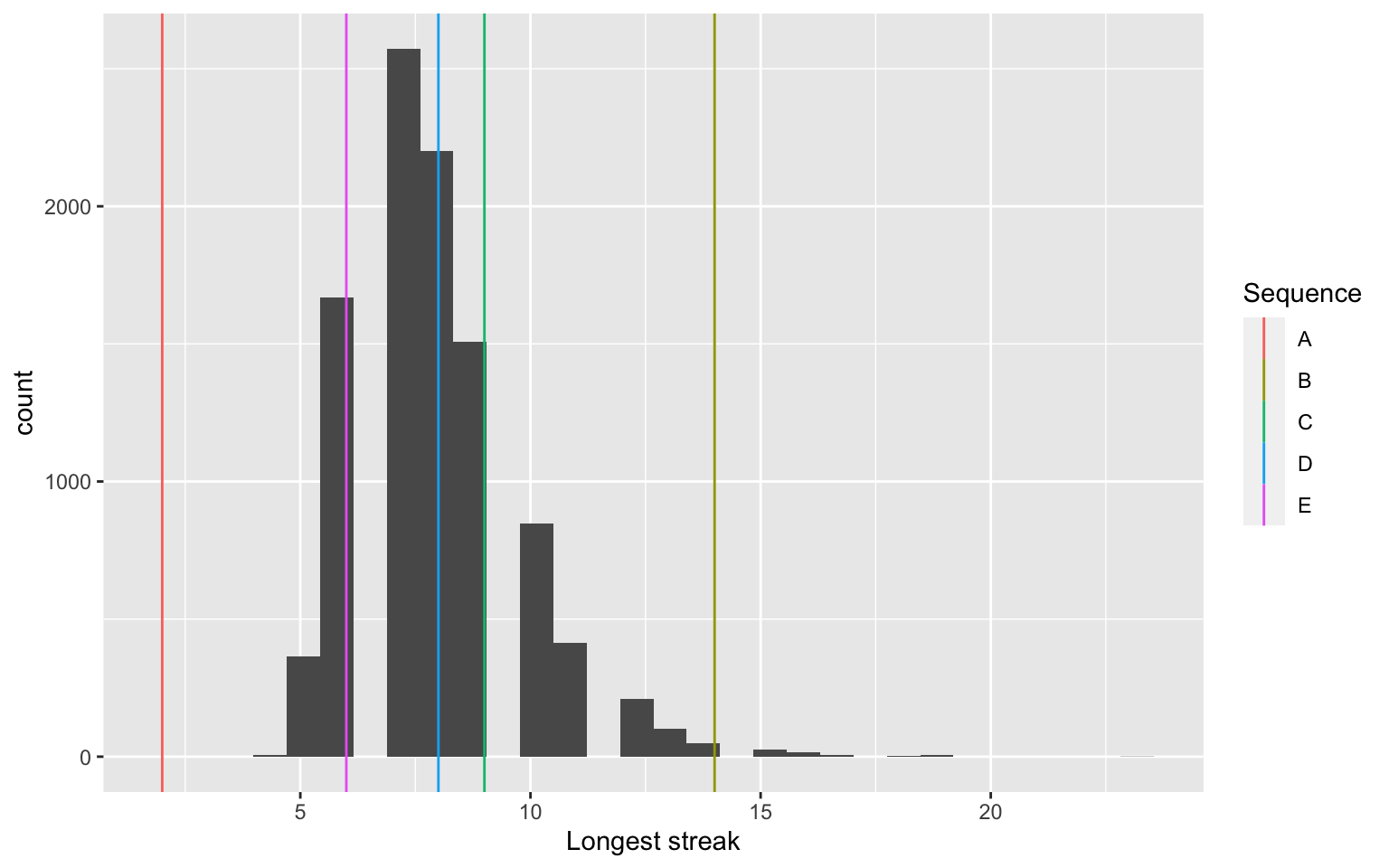
We can also consider a different test statistic: longest streak.

flip_streaks <- flips_long |>
  group_by(Sequence) |>
  summarize(longest_streak = max(rle(Flip)$length))
flip_streaks

# A tibble: 5 × 2
  Sequence longest_streak
  <chr>             <int>
1 A                     2
2 B                    14
3 C                     9
4 D                     8
5 E                     6

A slightly different test: streak length

We can then simulate the null distribution of streak length.

sim_streaks <- 
  data.frame(
    x = replicate(10000, 
                  max(rle(sample(c("H", "T"), size = 200, replace = T))$length)
    )
  )
ggplot() +
  geom_histogram(data = sim_streaks, aes(x = x), binwidth = 1) +
  geom_vline(data = flip_streaks,
             aes(color = Sequence, xintercept = longest_streak)) +
  xlab("Longest streak")

A slightly different test: streak length

Note that calculating the P-value is tricky here–a one-sided test may make the most sense.

p_vals <- sapply(flip_streaks$longest_streak,
                 function (x) mean(sim_streaks$x > x))
p_vals

[1] 1.0000 0.0057 0.1679 0.3186 0.7961

This suggests that the longest streaks are too long for sequence B. Note that we could try other test statistics. What about average streak length?

Designing your own hypothesis test

Come up with your own test statistic.
Simulate the null distribution of your test statistic.
Can you identify which sequence is the real one?

P-Hacking: Designing a test after seeing the data

In principle, we should decide which test to use before seeing the data. Why?

I could use the following test statistic: number of times the exact sequence \(D\) is obtained. What is the P-value for each sequence?