# A tibble: 6 × 5
  A     B     C     D     E
  <chr> <chr> <chr> <chr> <chr>
1 T     H     H     T     H
2 H     H     H     H     H
3 T     H     T     H     H
4 H     T     H     H     H
5 H     T     T     H     T
6 T H T T H MATH167R: Hypothesis Testing
Overview of today
- Simulations for power analysis
- P-hacking simulations
Designing your own hypothesis test
First, load the flips using the following code.
Can you tell which is real and which are fake?
Visual inspection
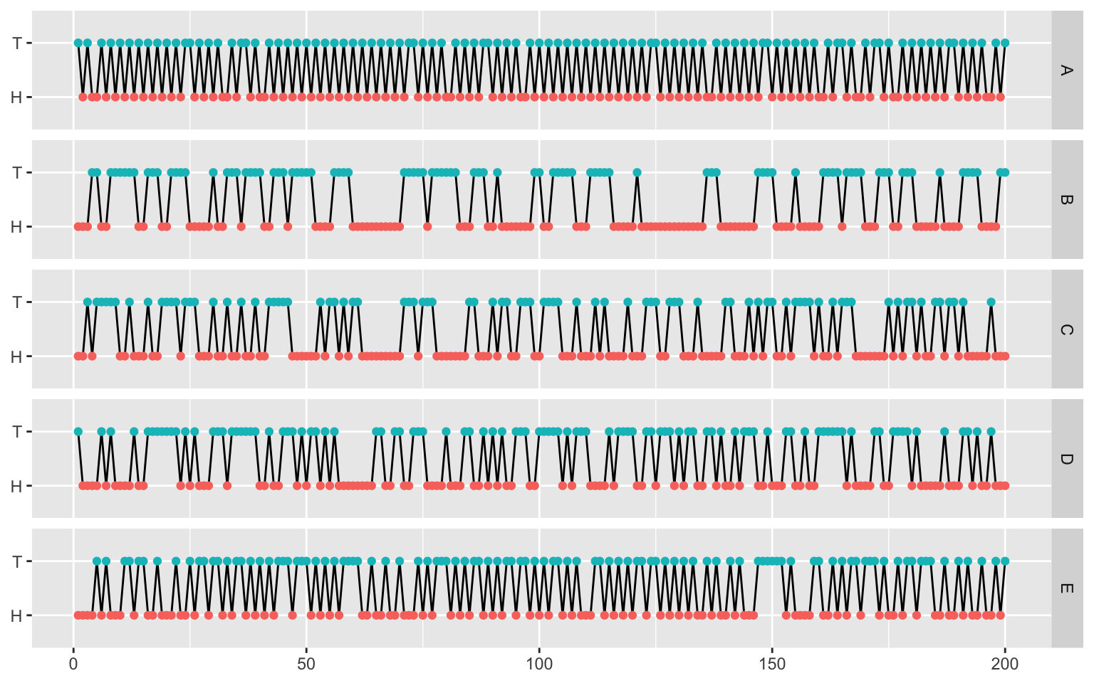
Visual inspection
flips_long <- flips |>
  mutate(id = 1:200) |>
  pivot_longer(-id,  names_to = "Sequence", values_to = "Flip")

flips_long |>
  ggplot(aes(x = id, y = Flip, group = Sequence)) +
  geom_line() +
  geom_point(aes(color = Flip)) +
  facet_grid(rows = vars(Sequence)) +
  theme(
    legend.position = "none",
    axis.title = element_blank()
  )
A slightly different test: streak length
We can also consider a different test statistic: longest streak.
A slightly different test: streak length
We can then simulate the null distribution of streak length.
Permutation tests
Typically, for hypothesis testing, we need to know the sampling distribution of the test statistic when the null hypothesis is true.
In some cases, we can derive the null sampling distribution analytically.
What if we don’t know the sampling distribution under the null? A permutation test is simple way to estimate the sampling distribution for any test statistic, requiring only some exchangeability assumptions on the data.
Permutation tests
Example: Suppose we want to understand whether carrying a particular genetic variant affects an individual’s height \(y\).
Permutation tests
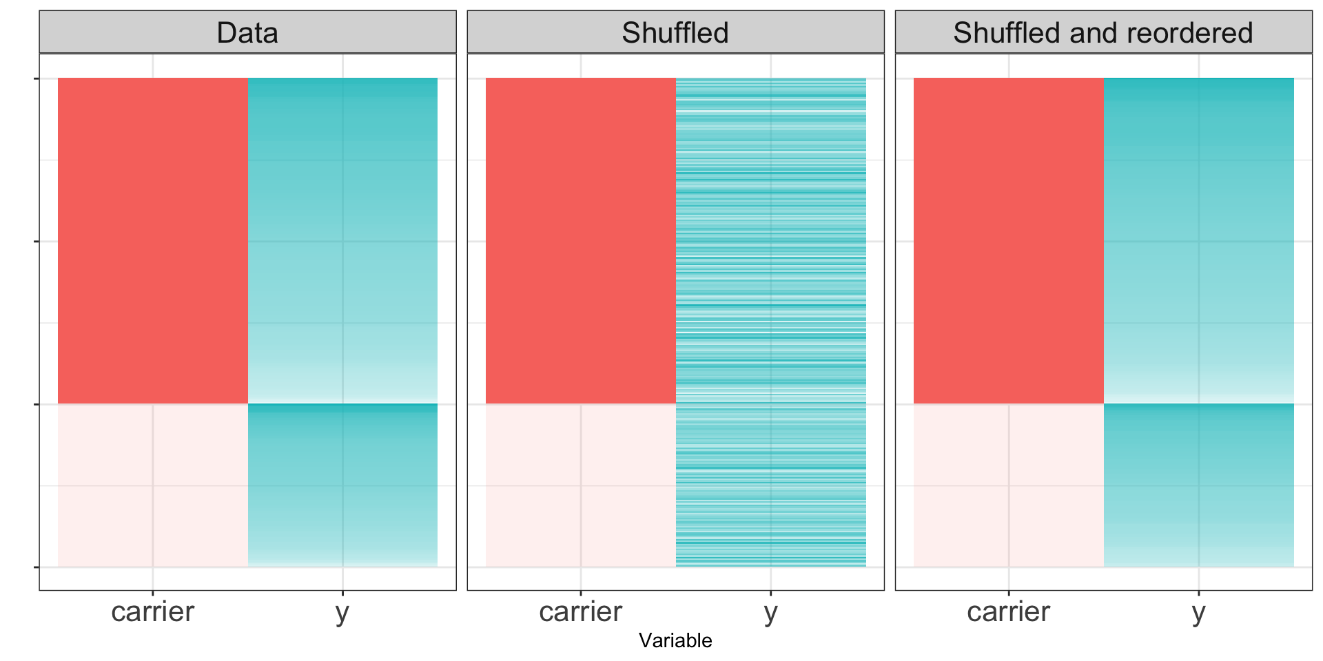
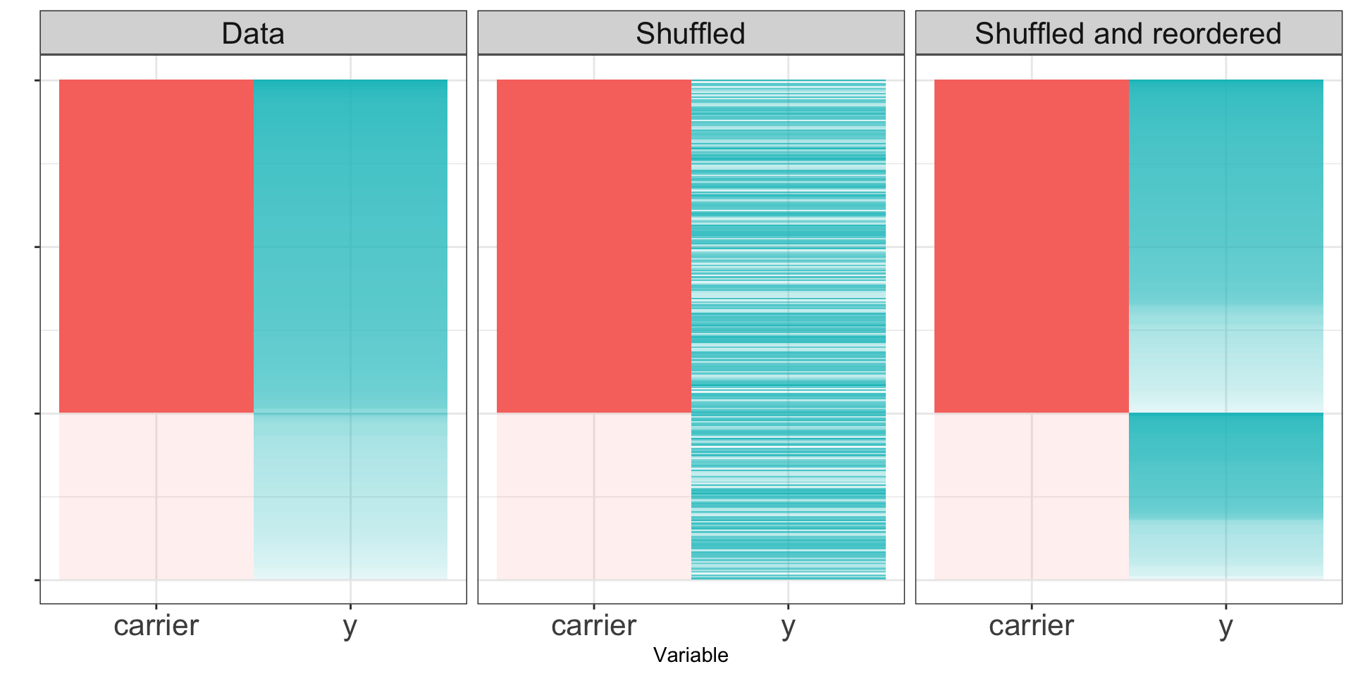
If the null hypothesis is true, the distribution of \(Y\) for the carriers should look the same as the distribution for the non-carriers. If we permute the labels repeatedly, we can get resampled datasets.
If the null hypothesis is true, the shuffled data sets will resemble the original dataset. If the null hypothesis is false, the shuffled dataset may not look like the real data.
Null hypothesis true
Null hypothesis false
Permutation tests
- Calculate a test statistic based on the observed data.
- Repeatedly permute the group labels to create resamples. For each resample, compute the resample test statistic.
- Compare the observed data test statistic with the distribution of resampled test statistics.
Permutation tests
In the case of our simulated data, we know the true distribution of the difference of sample means. We can thus use a \(t\)-test to perform our hypothesis test:
    Two Sample t-test

data:  null_y[carrier == 0] and null_y[carrier == 1]
t = -0.55208, df = 298, p-value = 0.5813
alternative hypothesis: true difference in means is not equal to 0
95 percent confidence interval:
 -0.3175650  0.1784227
sample estimates:
  mean of x   mean of y
-0.09674072 -0.02716956
Permutation tests
Compare with the \(t\)-test for the alternative hypothesis data:
    Two Sample t-test

data:  alt_y[carrier == 0] and alt_y[carrier == 1]
t = -41.762, df = 298, p-value < 2.2e-16
alternative hypothesis: true difference in means is not equal to 0
95 percent confidence interval:
 -5.246960 -4.774709
sample estimates:
 mean of x  mean of y
0.01439314 5.02522740
Permutation tests
For now, though, let’s pretend we don’t know the true null sampling distribution of our test statistic.
Permutation tests
[1] 0.546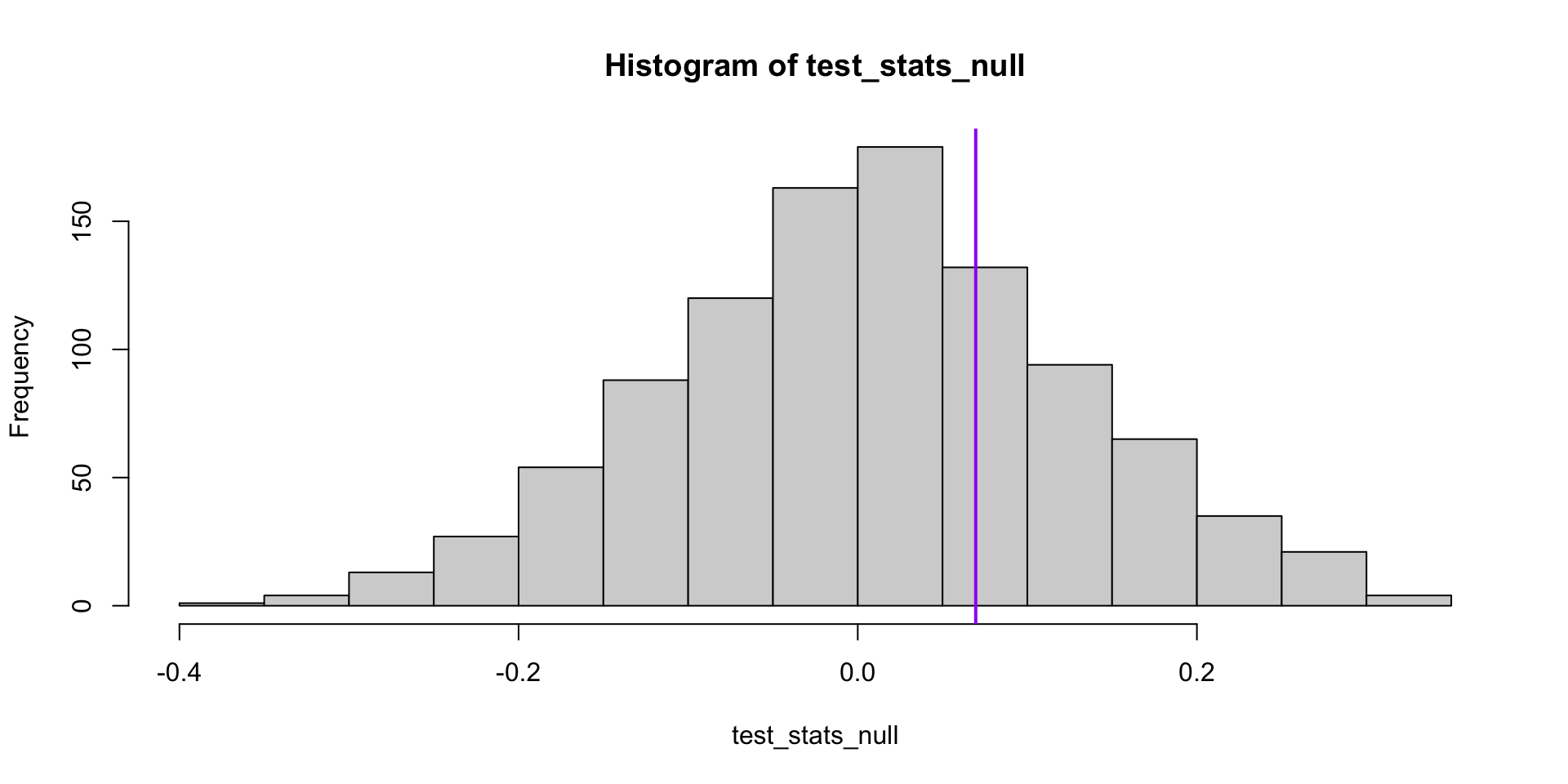
Permutation tests
Compare with the case where the null hypothesis is false.
set.seed(1)
alt_diff <- mean(alt_y[carrier==1]) - mean(alt_y[carrier==0])
test_stats_alt <- replicate(1000, single_test(carrier, alt_y))
hist(test_stats_alt, xlim = c(-0.5, 6))
abline(v = alt_diff, lwd=2, col="purple")[1] 0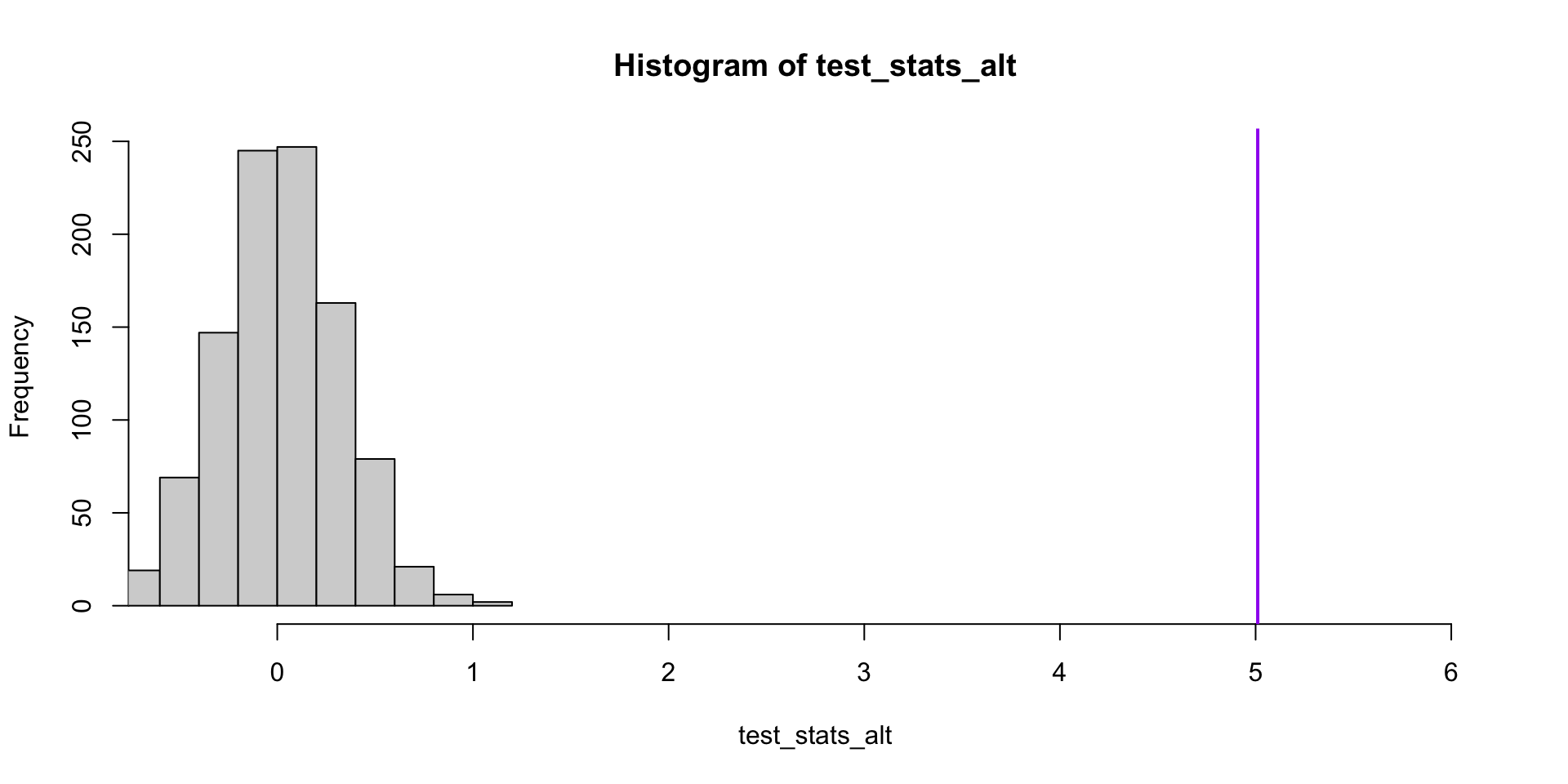
Permutation tests: sleep data
What if we apply this idea to the sleep data?
Permutation tests: sleep data
test_stat <- mean(sleep$extra[sleep$group == 1]) -
  mean(sleep$extra[sleep$group == 2])
single_test <- function(label, y) {
  resample <- sample(label)
  # resample test statistic
  mean(y[resample == 1]) - mean(y[resample == 2])
}
test_stats_alt <- replicate(1000, single_test(sleep$group, sleep$extra))
hist(test_stats_alt)
abline(v = test_stat, lwd=2, col="purple")[1] 0.099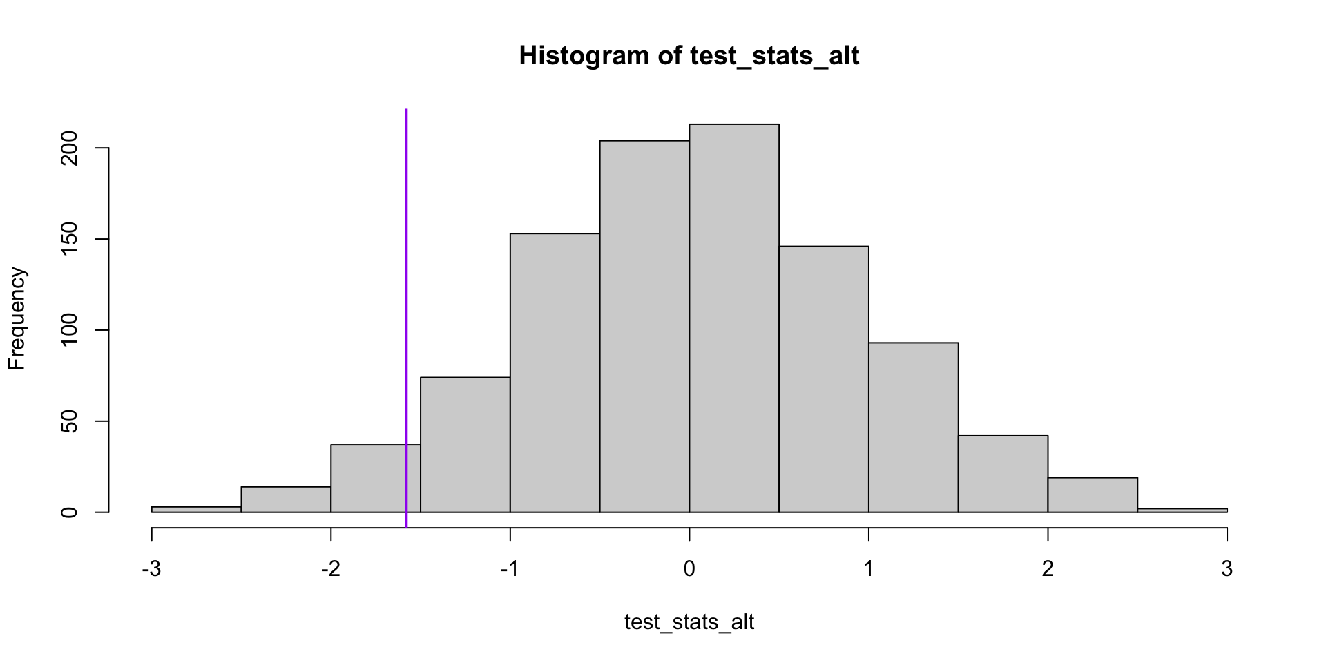
Power analysis
Recall that the power of a hypothesis test is the probability of rejecting the null hypothesis when the null hypothesis is false.
Note the power will depend on the size of the difference between the true sampling distribution and the null hypothesis sampling distribution.
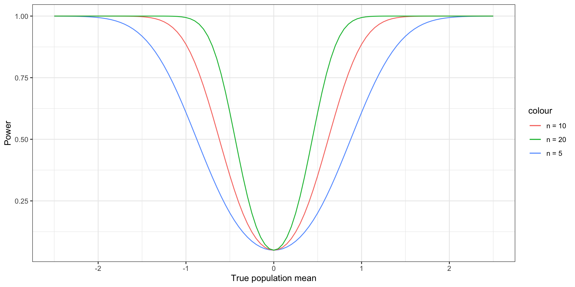
One sample \(z\)-test
Suppose that \(X_1,\ldots, X_n\sim N(\mu, 1)\).
Consider the hypotheses \(H_0:\mu=0\) and \(H_a:\mu\neq 0\).
We reject at the \(\alpha\) significance level if \[|\overline{X}_n| > \frac{z_{\alpha/2}}{\sqrt{n}}\]
If \(\mu=\mu_a\neq 0\), then \[\overline{X}_n\sim N\left(\mu_a, \frac{1}{\sqrt{n}}\right)\]
One sample \(z\)-test
\[ \begin{align} P\left(|\overline{X}_n| > \frac{z_{\alpha/2}}{\sqrt{n}}\right)&=P\left(\overline{X}_n> \frac{z_{\alpha/2}}{\sqrt{n}}\right) + P\left(\overline{X}_n < -\frac{z_{\alpha/2}}{\sqrt{n}}\right)\\ &=P\left(\frac{\overline{X}_n-\mu_a}{1/\sqrt{n}}> z_{\alpha/2}-\frac{\mu_a}{1/\sqrt{n}}\right) \\ &+ P\left(\frac{\overline{X}_n-\mu_a}{1/\sqrt{n}}<-z_{\alpha/2}-\frac{\mu_a}{1/\sqrt{n}}\right)\\ &=\left(1-\Phi\left(z_{\alpha/2}-\frac{\mu_a}{1/\sqrt{n}}\right)\right)+\Phi\left(-z_{\alpha/2}-\frac{\mu_a}{1/\sqrt{n}}\right) \end{align} \]
One sample \(z\)-test
one_sample_z_power <- function(mu_a, alpha, n) {
  z <- qnorm(1 - alpha / 2)
  return(1 - pnorm(z - mu_a * sqrt(n)) + pnorm(-z - mu_a * sqrt(n)))
}

# plot the power function
x <- data.frame(x = seq(-3, 3, length.out = 1000))
ggplot(x, aes(x = x)) +
  geom_function(fun = one_sample_z_power,
                aes(color = "n = 5"),
                args = list(alpha = .05, n = 5)) +
  geom_function(fun = one_sample_z_power,
                aes(color = "n = 10"),
                args = list(alpha = .05, n = 10)) +
  geom_function(fun = one_sample_z_power,
                aes(color = "n = 20"),
                args = list(alpha = .05, n = 20)) +
  xlab("True population mean") + ylab("Power") +
  theme_bw()
One sample \(z\)-test
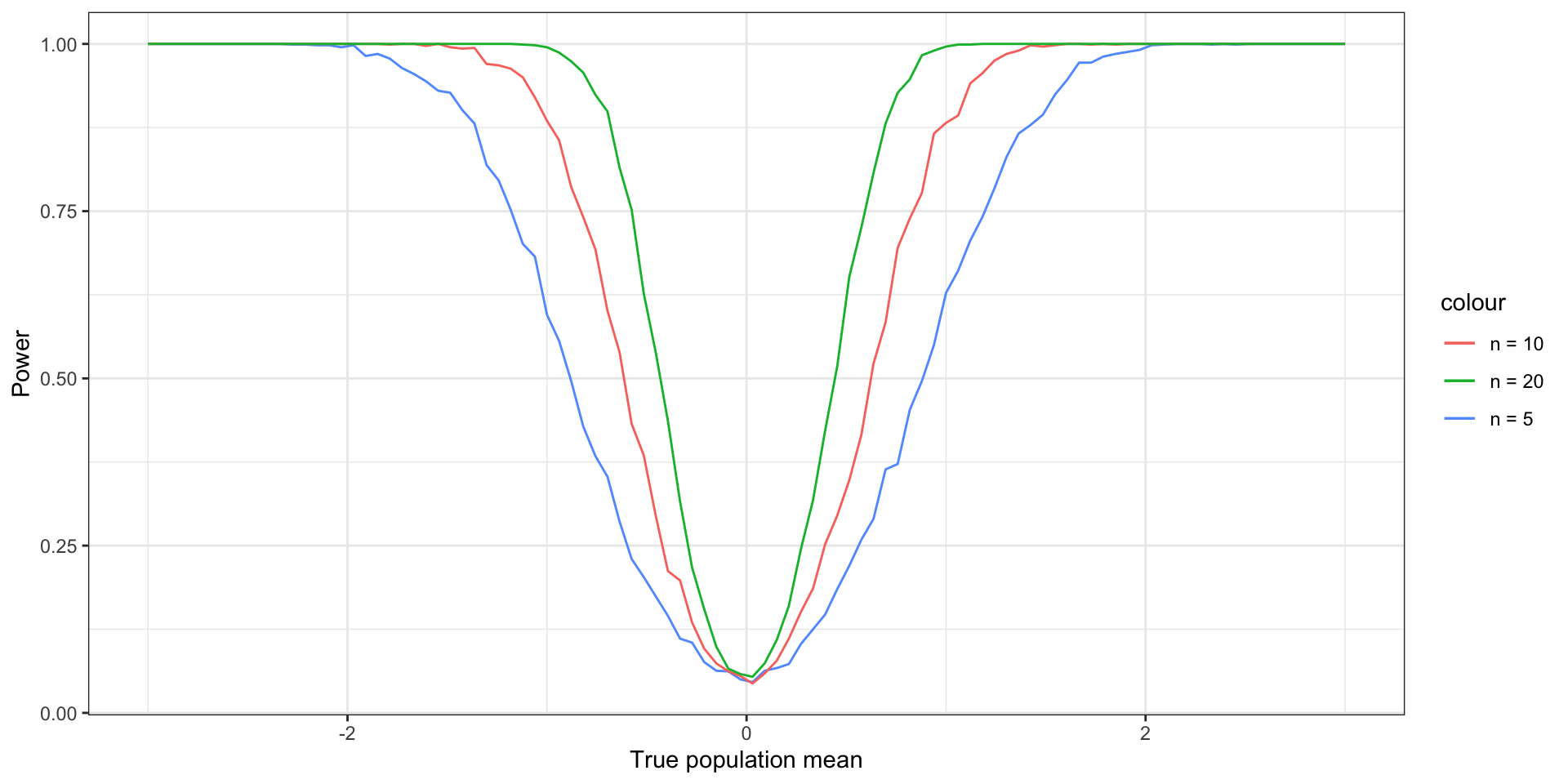
Using simulations to estimate power
simulate_test <- function(mu_a, alpha, n) {
  Xbar <- mean(rnorm(n, mean = mu_a, sd = 1))
  Z_score <- Xbar * sqrt(n)
  return(abs(Z_score) > qnorm(1 - alpha / 2))
}
power_sim <- function(mu_a, alpha, n) {
  return(mean(replicate(1000, simulate_test(mu_a, alpha, n))))
}

mu_a <- data.frame(mu_a = seq(-2.5, 2.5, length.out = 100))
sample_sizes <- c(5, 10, 20)

# matrix of simulation results
sim_results <-
  sapply(sample_sizes,
         function(n)
           sapply(mu_a$mu_a,
                  function(mu)
                    power_sim(mu, .05, n)))

ggplot(mu_a, aes(x = mu_a)) +
  geom_line(aes(y = sim_results[, 1], color = "n = 5")) +
  geom_line(aes(y = sim_results[, 2], color = "n = 10")) +
  geom_line(aes(y = sim_results[, 3], color = "n = 20")) +
  xlab("True population mean") + ylab("Power") +
  theme_bw()
Using simulations to estimate power
Exercise: estimating power
If \(X_1,\ldots X_n\sim N(1, 1)\), what is the power for a one-sample \(t\) test for the hypotheses \(H_0:\mu = 0\) and \(H_a:\mu\not=0\) if \(n=30\)?
Create a simulation to estimate the power.
P-hacking simulations
P-hacking refers to the practice of repeatedly performing hypothesis tests (and potentially manipulating the data) until a statistically significant P-values is obtained. Usually, only this final result is published, without mentioning all of the manipulations that came before.
P-hacking simulations
Suppose we simulate 25 observations of 8 variables which we know to be uncorrelated.
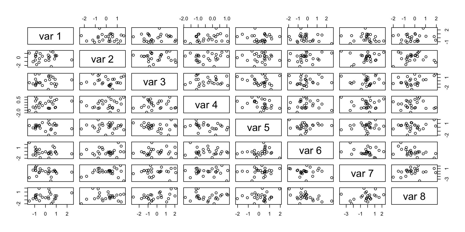
P-hacking simulations
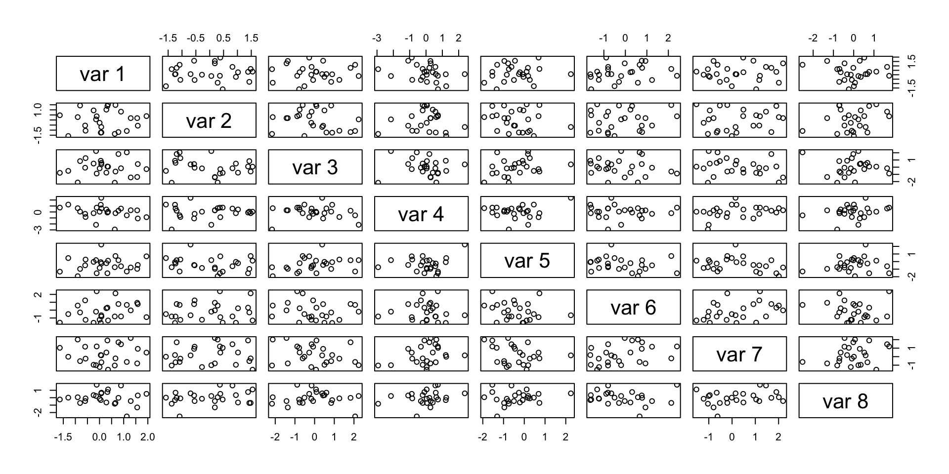
Multiple testing simulations
What if we perform a hypothesis test to test whether the correlation is zero between each pair of variables using cor.test()? With only 8 variables, we have 28 potential comparisons, the probability that we will (falsely) reject the null is already:
Multiple testing simulations
set.seed(1029)
no_signal_data<- matrix(rnorm(200), ncol = 8) # 25 x 8 matrix
pairs_to_compare <- combn(8, 2) # all combinations of 2 numbers from 1-8
p_values <- c()
for (i in 1:ncol(pairs_to_compare)) {
  index_1 <- pairs_to_compare[1, i]
  index_2 <- pairs_to_compare[2, i]
  test_res <-
    cor.test(no_signal_data[, index_1],
             no_signal_data[, index_2])
  p_values <- c(p_values, test_res$p.value)
}
print(min(p_values))
[1] 0.006656272Multiple testing simulations
For this reason it is common to perform a correction to the p-values when many hypothesis tests are conducted.
Example: The Bonferroni correction divides \(\alpha\) by the number of tests performed to get the corrected significance level.