MATH167R: Linear regression

Peter Gao

Overview of today

• Covariance and correlation
• Linear regression

Relating numerical variables

Covariance and correlation

In statistics, correlation and covariance usually refer to a specific type of association.

• If \(X\) and \(Y\) are linearly associated, then they are correlated.

Correlation

Correlation can also refer to the correlation coefficient.

The (Pearson) correlation coefficient \(R\) is a statistic between \(-1\) and 1 that describes the strength and direction of the linear relationship between two variables.

\[R = \frac{1}{n-1}\sum_{i=1}^n\frac{x_i-\overline{x}}{s_x}\frac{y_i-\overline{y}}{s_y}\]

The sign of \(R\) indicates the direction of the relationship. The absolute value of \(R\) indicates the strength.

Correlation and covariance

attach(mtcars)
cor(mpg, wt)

[1] -0.8676594

cov(mpg, wt)

[1] -5.116685

Pairs plots for assessing many relationships

pairs(~mpg + hp + wt, mtcars)

Regression methods

Assume we have some data:

• \(X_1,\ldots, X_p\): \(p\) independent variables/explanatory variables/covariates/predictors
• \(Y\): the dependent variables/response/outcome.

We want to know the relationship between our covariates and our response, we can do this with a method called regression. Regression provides us with a statistical method to conduct inference and prediction.

Regression methods

• inference: assess the relationship between our variables, our statistical model as a whole, predictor importance
  • What is the relationship between sleep and GPA?
  • Is parents’ education or parents’ income more important for explaining income?
• prediction: predict new/future outcomes from new/future covariates
  • Can we predict test scores based on hours spent studying?

Why is it called regression?

Simple linear regression

How does the speed of a car affect its stopping distance?

plot(dist ~ speed, data = cars,
     xlab = "Speed (mph)",
     ylab = "Stopping Distance (ft)",
     pch  = 16, col = "blue")

Simple linear regression

Suppose \(x_1,\ldots, x_n\) represent the speed values of each car in our dataset. Let \(Y_1,\ldots, Y_n\) represent the dist variable.

The simple linear regression model is given by \[Y_i=\beta_0+\beta_1x_i+\epsilon_i\] where:

• \(\beta_0\) is the intercept parameter

• \(\beta_1\) is the slope parameter

• \(\epsilon_i\) represents iid \(N(0,\sigma^2)\) errors, where \(\sigma^2\) is the variance of \(\epsilon_i\).

Simple linear regression

Under this model, we can also write that \[Y_i\mid X_i= x_i\sim N(\beta_0+\beta_1x_i, \sigma^2)\] As a result \[E(Y_i\mid X_i= x_i)= \beta_0+\beta_1x_i\] \[\mathrm{Var}(Y_i\mid X_i= x_i)= \sigma^2\]

Simple linear regression

Typically, we say there are four assumptions for simple linear regression:

• Linearity: The relationship between \(X\) and \(E(Y\mid X)\) is linear: \[E(Y_i\mid X_i= x_i)= \beta_0+\beta_1x_i\]
• Independence: The observations \(Y_1,\ldots, Y_n\) are independent of each other.
• Normality: \[Y_i\mid X_i= x_i\sim N(\beta_0+\beta_1x_i, \sigma^2)\]
• Equal variance: The variance of the errors \(\epsilon_i\) is the same for all values of \(x_i\).

Note that even if one or more of these assumptions breaks, linear regression can still be useful if used with caution.

Simple linear regression: Least squares

Typically, we start with data \(Y_1,\ldots, Y_n\) and \(x_1,\ldots, x_n\). How do we estimate \(\beta_0\) and \(\beta_1\)?

In other words, what is the best line to use for modeling the relationship between \(X\) and \(Y\)?

Usually, we use the least squares line, which is the solution to the following optimization problem: \[\arg\min\sum_{i=1}^n (y_i-(\beta_0+\beta_1x_i))^2=\arg\min\sum_{i=1}^n (y_i-\widehat{y}_i)^2\] where \(\widehat{y}_i\) is the model prediction for \(y_i\).

Simple linear regression: the lm function

lm_res = lm(dist ~ speed, data = cars)
lm_res

Call:
lm(formula = dist ~ speed, data = cars)

Coefficients:
(Intercept)        speed  
    -17.579        3.932  

Simple linear regression: the lm function

plot(dist ~ speed, data = cars,
     xlab = "Speed (mph)",
     ylab = "Stopping Distance (ft)", 
     pch  = 16, col  = "blue")
abline(lm_res,  col = "red")

Simple linear regression: Inference

For the simple linear regression model, typically we wish to carry out inference on \(\beta_1\). One way to do so is via a hypothesis test:

\(H_0:\beta_1=0\) \(H_a:\beta_1\not=0\)

summary(lm_res)

Call:
lm(formula = dist ~ speed, data = cars)

Residuals:
    Min      1Q  Median      3Q     Max 
-29.069  -9.525  -2.272   9.215  43.201 

Coefficients:
            Estimate Std. Error t value Pr(>|t|)    
(Intercept) -17.5791     6.7584  -2.601   0.0123 *  
speed         3.9324     0.4155   9.464 1.49e-12 ***
---
Signif. codes:  0 '***' 0.001 '**' 0.01 '*' 0.05 '.' 0.1 ' ' 1

Residual standard error: 15.38 on 48 degrees of freedom
Multiple R-squared:  0.6511,    Adjusted R-squared:  0.6438 
F-statistic: 89.57 on 1 and 48 DF,  p-value: 1.49e-12

Simple linear regression: Inference

We can also construct a confidence interval for \(\beta_1\) if our focus isn’t on developing evidence against any null hypothesis:

confint(lm_res)

                 2.5 %    97.5 %
(Intercept) -31.167850 -3.990340
speed         3.096964  4.767853

Simple linear regression: Prediction

Prediction generally involves estimating the value of new data \(Y_{n+1}\) given \(X_{n+1}\). We can use the predict() function with our lm() results:

predict(lm_res,
        newdata = list(speed = 19.5))

       1 
59.10288 

# get prediction interval
predict(lm_res, 
        newdata = list(speed = 19.5),
        interval = "prediction")

       fit      lwr      upr
1 59.10288 27.68517 90.52059

Simple linear regression: Prediction

Note that the predict() function can also be used to generate “confidence” intervals:

• interval = "prediction": Construct a confidence interval for \(Y_{n+1}|X_{n+1}=x_{n+1}\), the value of a new observation for which \(X_{n+1}=x_{n+1}\)
• interval = "confidence": Construct a confidence interval for \(E(Y_{n+1}|X_{n+1}=x_{n+1})\), the value of the conditional mean when \(X_{n+1}=x_{n+1}\)

Simple linear regression: Prediction

# prediction interval
predict(lm_res, 
        newdata = list(speed = 19.5),
        interval = "prediction")

       fit      lwr      upr
1 59.10288 27.68517 90.52059

# confidence interval
predict(lm_res, 
        newdata = list(speed = 19.5),
        interval = "confidence")

       fit      lwr     upr
1 59.10288 53.54796 64.6578

Warm-up

What is the method of least squares and how does it relate to linear regression?

Classify the following questions as inference or prediction:

1. Can we use high school students’ SAT/ACT scores to estimate their college GPAs?
2. Is there an association between political candidates’ heights and the number of votes they receive?
3. Do states with higher minimum wages have lower poverty rates?

Simple linear regression: Checking assumptions

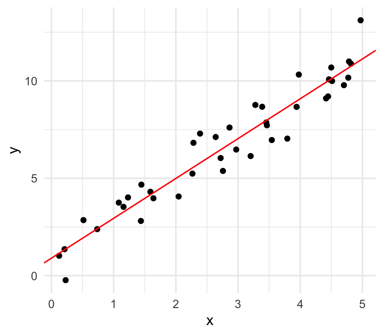
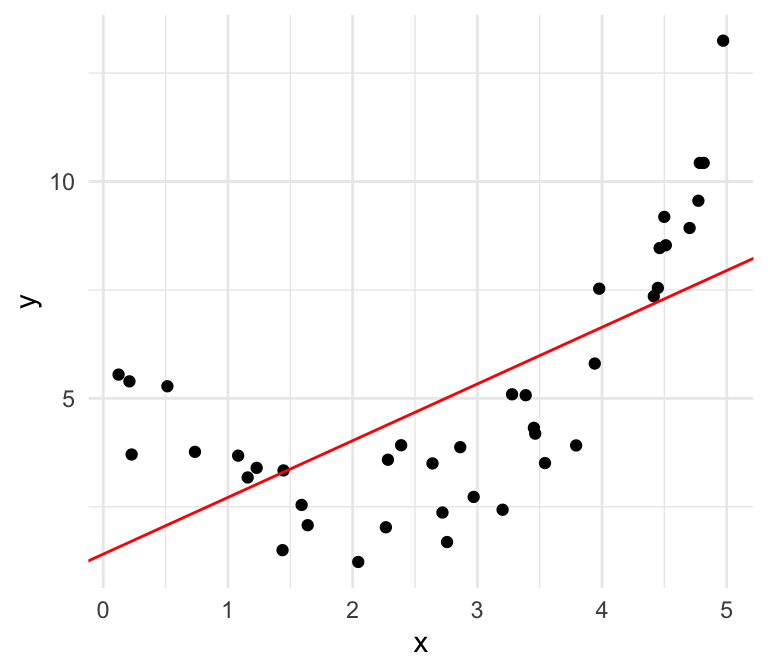
Typically, we say there are four assumptions for simple linear regression:

• Linearity: The relationship between \(X\) and \(E(Y\mid X)\) is linear: \[E(Y_i\mid X_i= x_i)= \beta_0+\beta_1x_i\]
• Independence: The observations \(Y_1,\ldots, Y_n\) are independent of each other.
• Normality: \[Y_i\mid X_i= x_i\sim N(\beta_0+\beta_1x_i, \sigma^2)\]
• Equal variance: The variance of the errors \(\epsilon_i\) is the same for all values of \(x_i\).

Checking linearity

Linear

Nonlinear

Checking linearity with residual plot

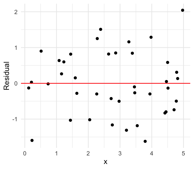
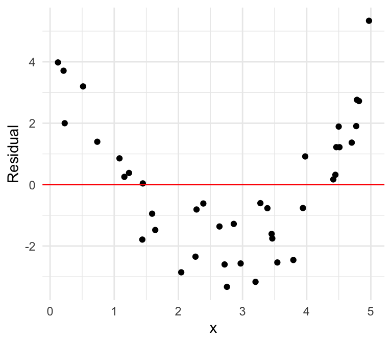
We can also plot the residuals against our independent variable, where we define the residual as follows: \[\widehat{\epsilon}_i = \mathrm{Residual} = \mathrm{Observed} - \mathrm{Predicted}=y -\widehat{y}\]

Checking linearity with residual plot

Linear

Nonlinear

Checking independence

Checking independence is typically more difficult. We require that conditional on the dependent variables \(x_1,\ldots, x_n\), the response variables \(Y_1,\ldots, Y_n\) are independent.

Example of independence: survey data obtained via simple random sampling

Example of dependence: height and weight measurements of penguins, where each penguin is measured twice

Checking normality of errors

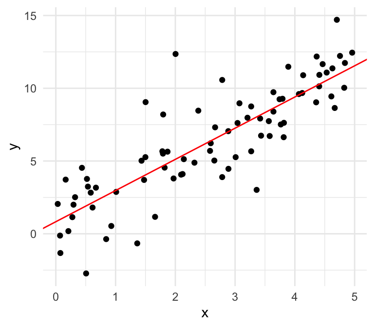
Can you spot the difference?

Normal errors

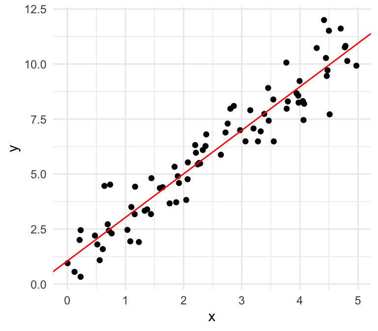
Non-normal errors

Checking normality of errors with quantile-quantile plot

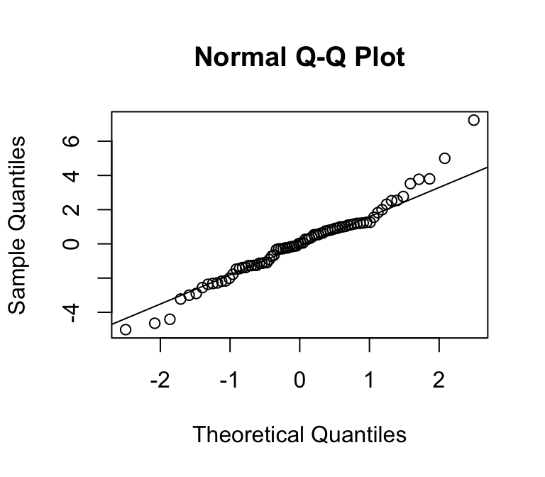
We can use a quantile-quantile plot to see whether our estimated residuals are approximately normally distributed.

lm_res <- lm(dist ~ speed, cars)
qqnorm(resid(lm_res))
qqline(resid(lm_res))

Checking normality of errors with quantile-quantile plot

What do you notice?

Checking normality of errors with quantile-quantile plot

Normal errors

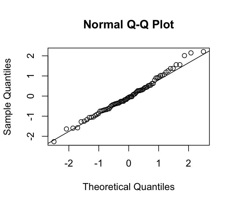
Non-normal errors

Checking equal variances (homoskedasticity)

Can you spot the difference?

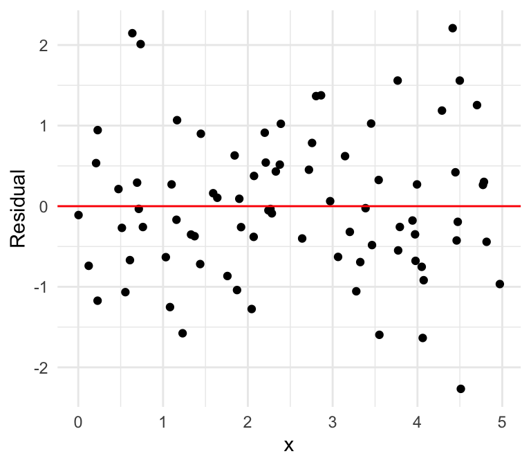
Equal variances

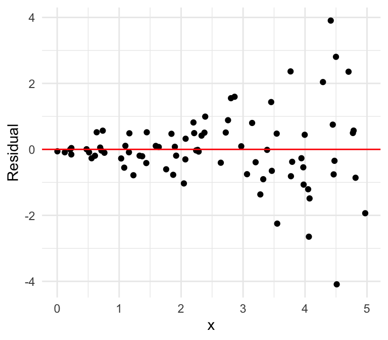
Unequal variances

Checking equal variances (homoskedasticity) with residual plot

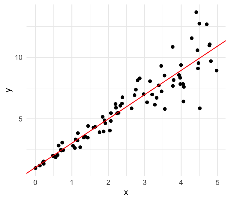
Can you spot the difference using the residual plot?

Equal variances

Unequal variances

Multiple linear regression

What if we have multiple input variables?

data(mtcars)
head(mtcars)

                   mpg cyl disp  hp drat    wt  qsec vs am gear carb
Mazda RX4         21.0   6  160 110 3.90 2.620 16.46  0  1    4    4
Mazda RX4 Wag     21.0   6  160 110 3.90 2.875 17.02  0  1    4    4
Datsun 710        22.8   4  108  93 3.85 2.320 18.61  1  1    4    1
Hornet 4 Drive    21.4   6  258 110 3.08 3.215 19.44  1  0    3    1
Hornet Sportabout 18.7   8  360 175 3.15 3.440 17.02  0  0    3    2
Valiant           18.1   6  225 105 2.76 3.460 20.22  1  0    3    1

Multiple linear regression

Given our response \(Y\) and our predictors \(X_1, \ldots, X_p\), a linear regression model takes the form:

\[ \begin{align} Y &= \beta_0 + \beta_1 X_1 + \cdots + \beta_p X_p + \epsilon,\\ \epsilon &\sim N(0,\sigma^2) \end{align} \]

Note: If we wish to include a categorical covariate, we can add indicator variables for each category.

Multiple linear regression

\[ \begin{align} Y &= \beta_0 + \beta_1 X_1 + \cdots + \beta_p X_p + \epsilon,\\ \epsilon &\sim N(0,\sigma^2) \end{align} \]

• \(Y\): dependent variable, outcome, response
• \(X_j\): independent variable, covariate, predictor
• \(\beta_0\): Intercept
• \(\beta_j\): coefficient, the expected difference in the response between two observations differing by one unit in \(X_j\), with all other covariates identical.
• \(\epsilon\): error, noise, with mean \(0\) and variance \(\sigma^2\)

Multiple linear regression: example

Consider the following example using the penguins data.

library(palmerpenguins)
data(penguins)
head(penguins)

# A tibble: 6 × 8
  species island    bill_length_mm bill_depth_mm flipper_length_mm body_mass_g
  <fct>   <fct>              <dbl>         <dbl>             <int>       <int>
1 Adelie  Torgersen           39.1          18.7               181        3750
2 Adelie  Torgersen           39.5          17.4               186        3800
3 Adelie  Torgersen           40.3          18                 195        3250
4 Adelie  Torgersen           NA            NA                  NA          NA
5 Adelie  Torgersen           36.7          19.3               193        3450
6 Adelie  Torgersen           39.3          20.6               190        3650
# ℹ 2 more variables: sex <fct>, year <int>

Multiple linear regression: example

Suppose we are interested in predicting body_mass_g using flipper_length_mm.

ggplot(penguins, mapping = aes(x = flipper_length_mm, y = body_mass_g)) +
  geom_point() +
  geom_smooth(method = "lm")

Multiple linear regression: example

lm_res <- lm(body_mass_g ~ flipper_length_mm, data = penguins)
summary(lm_res)

Call:
lm(formula = body_mass_g ~ flipper_length_mm, data = penguins)

Residuals:
     Min       1Q   Median       3Q      Max 
-1058.80  -259.27   -26.88   247.33  1288.69 

Coefficients:
                   Estimate Std. Error t value Pr(>|t|)    
(Intercept)       -5780.831    305.815  -18.90   <2e-16 ***
flipper_length_mm    49.686      1.518   32.72   <2e-16 ***
---
Signif. codes:  0 '***' 0.001 '**' 0.01 '*' 0.05 '.' 0.1 ' ' 1

Residual standard error: 394.3 on 340 degrees of freedom
  (2 observations deleted due to missingness)
Multiple R-squared:  0.759, Adjusted R-squared:  0.7583 
F-statistic:  1071 on 1 and 340 DF,  p-value: < 2.2e-16

Multiple linear regression: example

Consider the following residual plot, where we define the residual as follows: \[\mathrm{Residual} = \mathrm{Observed} - \mathrm{Predicted}=y -\widehat{y}\]

Multiple linear regression: example

What if I also want to include species in the model? There are a few ways to do so.

Multiple linear regression: Group intercepts

The first way is to add species into the formula for our linear regression model:

lm_species_res <- lm(body_mass_g ~ flipper_length_mm + species,
                     data = penguins)
summary(lm_species_res)

Call:
lm(formula = body_mass_g ~ flipper_length_mm + species, data = penguins)

Residuals:
    Min      1Q  Median      3Q     Max 
-927.70 -254.82  -23.92  241.16 1191.68 

Coefficients:
                   Estimate Std. Error t value Pr(>|t|)    
(Intercept)       -4031.477    584.151  -6.901 2.55e-11 ***
flipper_length_mm    40.705      3.071  13.255  < 2e-16 ***
speciesChinstrap   -206.510     57.731  -3.577 0.000398 ***
speciesGentoo       266.810     95.264   2.801 0.005392 ** 
---
Signif. codes:  0 '***' 0.001 '**' 0.01 '*' 0.05 '.' 0.1 ' ' 1

Residual standard error: 375.5 on 338 degrees of freedom
  (2 observations deleted due to missingness)
Multiple R-squared:  0.7826,    Adjusted R-squared:  0.7807 
F-statistic: 405.7 on 3 and 338 DF,  p-value: < 2.2e-16

Multiple linear regression: Group intercepts

In this case, the model is as follows: \[Y=\beta_0+\beta_1x_1+\beta_2x_2+\beta_3x_3+\epsilon_i\] where:

• \(Y\) is body_mass_g
• \(x_1\) is flipper_length_mm
• \(x_2\) is a dummy variable equal to 1 if the penguin is Chinstrap and 0 otherwise.
• \(x_3\) is a dummy variable equal to 1 if the penguin is Gentoo and 0 otherwise.

What happened to the Adelie penguins?

Multiple linear regression: Group intercepts

When including a categorical variable in a linear regression model, R automatically treats one category as the reference group.

The value of the intercept \(\beta_0\) thus represents the expected value of \(Y\) when \(x_1\) is zero for an Adelie penguin.

How do we interpret the other \(\beta\) parameters?

Multiple linear regression: Group intercepts

• \(\beta_1\) represents the expected change in \(Y\) when flipper length increases by 1 mm.
• \(\beta_2+\beta_0\) represents the expected value of \(Y\) when \(x_1\) is zero for a Chinstrap penguin.
• \(\beta_2+\beta_0\) represents the expected value of \(Y\) when \(x_1\) is zero for a Gentoo penguin.

Multiple linear regression: Group intercepts

This model thus yields three parallel lines, one for each group.

Multiple linear regression: example

Now we obtain the following residual plot:

Multiple linear regression: Group-specific slopes

The previous model gave us group-specific intercepts, resulting in parallel lines. What if we want to let the slope vary across each species?

Multiple linear regression: Group-specific slopes

The standard approach is to introduce interaction terms:

lm_int_res <- lm(body_mass_g ~ flipper_length_mm * species,
                     data = penguins)
summary(lm_int_res)

Call:
lm(formula = body_mass_g ~ flipper_length_mm * species, data = penguins)

Residuals:
    Min      1Q  Median      3Q     Max 
-911.18 -251.93  -31.77  197.82 1144.81 

Coefficients:
                                    Estimate Std. Error t value Pr(>|t|)    
(Intercept)                        -2535.837    879.468  -2.883  0.00419 ** 
flipper_length_mm                     32.832      4.627   7.095 7.69e-12 ***
speciesChinstrap                    -501.359   1523.459  -0.329  0.74229    
speciesGentoo                      -4251.444   1427.332  -2.979  0.00311 ** 
flipper_length_mm:speciesChinstrap     1.742      7.856   0.222  0.82467    
flipper_length_mm:speciesGentoo       21.791      6.941   3.139  0.00184 ** 
---
Signif. codes:  0 '***' 0.001 '**' 0.01 '*' 0.05 '.' 0.1 ' ' 1

Residual standard error: 370.6 on 336 degrees of freedom
  (2 observations deleted due to missingness)
Multiple R-squared:  0.7896,    Adjusted R-squared:  0.7864 
F-statistic: 252.2 on 5 and 336 DF,  p-value: < 2.2e-16

Multiple linear regression: Group-specific slopes

The standard approach is to introduce interaction terms:

\[Y=\beta_0+\beta_1x_1+\beta_2x_2+\beta_3x_3+\beta_4(x_1 * x_2) + \beta_5(x_1*x_3)+\epsilon_i\] where:

• \(\beta_1\) is now the slope for our reference group (Adelie)
• \(\beta_1+\beta_4\) is the slope for Chinstrap
• \(\beta_1+\beta_5\) is the slope for Gentoo

Linear Regression

We can fully write out a linear regression model

\[ \begin{equation} \begin{bmatrix} y_1 \\ y_2\\ \vdots \\ y_n \end{bmatrix} = \begin{bmatrix} 1 & x_{1,1} & \cdots & x_{1,k}\\ 1 & x_{2,1} & \cdots & x_{2, k}\\ \vdots & \vdots & \ddots & \vdots \\ 1 & x_{n,1} & \cdots & x_{n, k}\end{bmatrix} \begin{bmatrix} \beta_0 \\ \beta_1 \\ \vdots \\ \beta_{k} \end{bmatrix} + \begin{bmatrix} \epsilon_1 \\ \epsilon_2 \\ \vdots \\ \epsilon_{n} \end{bmatrix} \end{equation} \]

Matrix Notation

This can also be expressed in matrix form:

\[ \begin{align} \mathbf{Y} &= \mathbf{X}\beta + \epsilon,\\ \epsilon &\sim N(0,1) \end{align} \]

• \(\mathbf{Y} \in \mathbb{R}^{n \times 1}\): an n-dimensional vector of the response
• \(\mathbf{X} \in \mathbb{R}^{n \times (k+1)}\): a \(((k+1)\times n)\) matrix of the predictors (including intercept)
• \(\beta \in \mathbb{R}^{((k+1)\times 1)}\): a \((k+1)\)-dimensional vector of regression parameters
• \(\epsilon \in \mathbb{R}^{n \times 1}\): an n-dimensional vector of the error term

\(\large \epsilon\): Error term

\(\epsilon\), pronounced epsilon, represents the error term of our model. We can model \(Y\) as a linear function of the \(X\)’s, but in the real world, the relationship won’t always be perfect. There is noise! It can come from

• Measurement error in the \(X\)’s
• Measurement error in the \(Y\)’s
• Unobserved/missing variables in the model
• Deviations in the true model from linearity
• True randomness

In linear regression, we assume that this error term is normally distributed with mean zero and variance \(\sigma^2\).

\(\beta_0\): Intercept

\(\beta_0\) is the intercept term of our model. Notice that

\[\mathbb{E}[Y|X_1 = X_2 = \cdots = X_p = 0] = \beta_0\]

Thus, \(\beta_0\) is the expected value of our response if all the covariates are equal to \(0\). This is also known as the y-intercept of our model.

\(X_j\): Independent variable

\(X_j\) represents the \(j\)^th independent variable in our model. Notice that \[\mathbb{E}[Y|X_1,\ldots, X_p] = \beta_0 + \beta_1 X_1 + \cdots + \beta_p X_p\] What happens to this expectation if we increase \(X_j\) by 1 unit, holding everything else constant?

The conditional expectation of \(Y\) increases by \(\beta_j\).

\(\beta_j\): Coefficient

\(\beta_j\) represents the \(j\)^th regression coefficient in our model. From the previous slide, we saw that for every 1 unit increase in \(X_j\), holding all other variables constant, the expected value of the response increases by \(\beta_j\). From this we can derive an interpretation.

Interpretation of \(\beta_j\): the expected difference in the response between two observations differing by one unit in \(X_j\), with all other covariates identical.

lm(): Linear Model

We fit a linear regression model in R using lm(). The first argument is a formula, which is a type of R object. Formulas typically take the following form: Y ~ X_1 + X_2 + ... + X_p.

The dependent variable, Y goes on the left-hand side of the tilde ~, which marks the formula. The independent variables are added on the right-hand side. Using this formula will give us a model in the form of

\[ \begin{align} Y &= \beta_0 + \beta_1 X_1 + \cdots + \beta_p X_p + \epsilon,\\ \epsilon &\sim N(0,\sigma^2) \end{align} \]

lm(): Linear Model

data(mtcars)
my_lm <- lm(mpg ~ hp + wt, data = mtcars)
class(my_lm)

[1] "lm"

my_lm

Call:
lm(formula = mpg ~ hp + wt, data = mtcars)

Coefficients:
(Intercept)           hp           wt  
   37.22727     -0.03177     -3.87783  

lm(): Linear Model

We can see from names() that lm objects contain a lot more than they print out by default.

names(my_lm)

 [1] "coefficients"  "residuals"     "effects"       "rank"         
 [5] "fitted.values" "assign"        "qr"            "df.residual"  
 [9] "xlevels"       "call"          "terms"         "model"        

summary() Model summaries

summary() or summary.lm() gives us a summary of our lm object in R.

• The quantiles of the residuals: hopefully, they match a normal distribution.
• Coefficients, their standard errors, and their individual significances
• (Adjusted) R-squared value: how much of the overall variability in the response is explained by the model?
• F-statistic: hypothesis test for the significance of the overall model

summary() Model summaries

summary(my_lm)

Call:
lm(formula = mpg ~ hp + wt, data = mtcars)

Residuals:
   Min     1Q Median     3Q    Max 
-3.941 -1.600 -0.182  1.050  5.854 

Coefficients:
            Estimate Std. Error t value Pr(>|t|)    
(Intercept) 37.22727    1.59879  23.285  < 2e-16 ***
hp          -0.03177    0.00903  -3.519  0.00145 ** 
wt          -3.87783    0.63273  -6.129 1.12e-06 ***
---
Signif. codes:  0 '***' 0.001 '**' 0.01 '*' 0.05 '.' 0.1 ' ' 1

Residual standard error: 2.593 on 29 degrees of freedom
Multiple R-squared:  0.8268,    Adjusted R-squared:  0.8148 
F-statistic: 69.21 on 2 and 29 DF,  p-value: 9.109e-12

plot(): Regression model diagnostics

Calling plot(my_lm) will return several diagnostic plots. Remember that we want our error term to look normally distributed with mean zero. We won’t go into all the details for this class, but here are some tips:

• Residuals vs Fitted: these are your errors (residuals) plotted over the predicted outcome (fitted). Errors should be random, so here you want to see randomly scattered points with no discernable pattern. You want the trend line to be approximately horizontal.
• Normal Q-Q plot: These are the quantiles of your errors against the quantiles of a normal distribution. In theory, your errors should be normally distributed, so you are hoping that points are mostly along the 45-degree \(y=x\) line.

plot(): Regression model diagnostics

• Scale-location: This looks at the magnitude of standardized residuals over the predicted outcome. Similar interpretation as residuals vs fitted. This can make it slightly easier to identify undesireable patterns.
• Residuals vs leverage: This can help identify highly influential points, such as outliers. If points are outside dotted red lines, then removing them would noticeably alter your results. Never just remove outliers! If it’s real data, it’s valid and removing it will bias your results. It is much more important to understand why outliers are there than to remove them.

plot(): Regression model diagnostics

plot(my_lm)

plot(): Regression model diagnostics

plot(): Regression model diagnostics

plot(): Regression model diagnostics

coef(): Extract coefficients

Use coef() to extract estimated coefficients as a vector.

coef(my_lm)

(Intercept)          hp          wt 
37.22727012 -0.03177295 -3.87783074 

fitted() Extract fitted values

Use fitted() to extract the fitted/estimated values for the response. This can be useful to compare how our fitted values compare to the estimated values to help assess model fit.

library(ggplot2)
mod_fits <- fitted(my_lm)
my_df <- data.frame(actual = mtcars$mpg, fitted = mod_fits)
ggplot(my_df, aes(x = fitted, y = actual)) +
  geom_point() +
  geom_abline(slope = 1, intercept = 0, col = "red", lty = 2) + 
  theme_bw(base_size = 15) +
  labs(x = "Fitted values", y = "Actual values", title = "Actual vs. Fitted") +
  theme(plot.title = element_text(hjust = 0.5))

fitted() Extract fitted values

predict(): Predict new outcomes

Use predict() to predict new outcomes given new explanatory variables. For example, pretend we observe two new cars with horsepowers of 100 and 150, respectively, and weights of 3000 and 3500, respectively.

# Note: wt is in 1000s of lbs
new_obs <- data.frame(hp = c(100, 150), wt = c(3, 3.5))
predict(my_lm, new_obs)

       1        2 
22.41648 18.88892 

We’ll come back to prediction in future lectures.

residuals(): Compute residuals

Use residuals() to compute the residuals for fitted values.

residuals(my_lm)

          Mazda RX4       Mazda RX4 Wag          Datsun 710      Hornet 4 Drive 
        -2.57232940         -1.58348256         -2.47581872          0.13497989 
  Hornet Sportabout             Valiant          Duster 360           Merc 240D 
         0.37273336         -2.37381631         -1.29904236          1.51293266 
           Merc 230            Merc 280           Merc 280C          Merc 450SE 
         0.80632669         -0.77945988         -2.17945988          0.67463146 
         Merc 450SL         Merc 450SLC  Cadillac Fleetwood Lincoln Continental 
         0.25616901         -1.64993945          0.04479541          1.03726743 
  Chrysler Imperial            Fiat 128         Honda Civic      Toyota Corolla 
         5.50751301          5.80097202          1.08761978          5.85379085 
      Toyota Corona    Dodge Challenger         AMC Javelin          Camaro Z28 
        -3.08644148         -3.31136386         -3.94097947         -1.25202805 
   Pontiac Firebird           Fiat X1-9       Porsche 914-2        Lotus Europa 
         2.44325481         -0.32665313         -0.03737415          2.63023081 
     Ford Pantera L        Ferrari Dino       Maserati Bora          Volvo 142E 
        -0.74648866         -1.22541324          2.26052287         -1.58364943 

Manipulating formulas

Working with formulas in R can be somewhat confusing, so it is important to understand how formulas work to make sure you are fitting the intended model.

- 1

Use - 1 to remove an intercept from your model. Only do this if you are very sure that what you are doing is appropriate. I don’t recommend doing this in practice.

no_intercept <- lm(mpg ~ hp + wt - 1, data = mtcars)
summary(no_intercept)

Call:
lm(formula = mpg ~ hp + wt - 1, data = mtcars)

Residuals:
    Min      1Q  Median      3Q     Max 
-19.407  -2.382   2.511   7.091  23.885 

Coefficients:
   Estimate Std. Error t value Pr(>|t|)   
hp -0.03394    0.03940  -0.861   0.3959   
wt  6.84045    1.89425   3.611   0.0011 **
---
Signif. codes:  0 '***' 0.001 '**' 0.01 '*' 0.05 '.' 0.1 ' ' 1

Residual standard error: 11.32 on 30 degrees of freedom
Multiple R-squared:  0.7264,    Adjusted R-squared:  0.7082 
F-statistic: 39.83 on 2 and 30 DF,  p-value: 3.599e-09

: operator

Use X1:X2 to include an interaction effect in your model. This is useful if you have reason to believe two covariates interact, such as gender and education in a wage model. In our case, we’ll assume horsepower and weight interact in their effect on mpg.

Typically (always?), if you include an interaction effect, you should also include the marginal effects. You can do this automatically using X1*X2.

: operator

interact <- lm(mpg ~ hp:wt, data = mtcars)
summary(interact)

Call:
lm(formula = mpg ~ hp:wt, data = mtcars)

Residuals:
    Min      1Q  Median      3Q     Max 
-4.8831 -2.0952 -0.4577  1.2262  7.9282 

Coefficients:
             Estimate Std. Error t value Pr(>|t|)    
(Intercept) 27.745642   1.062236   26.12  < 2e-16 ***
hp:wt       -0.014872   0.001727   -8.61 1.32e-09 ***
---
Signif. codes:  0 '***' 0.001 '**' 0.01 '*' 0.05 '.' 0.1 ' ' 1

Residual standard error: 3.288 on 30 degrees of freedom
Multiple R-squared:  0.7119,    Adjusted R-squared:  0.7023 
F-statistic: 74.14 on 1 and 30 DF,  p-value: 1.321e-09

* operator

interact <- lm(mpg ~ hp*wt, data = mtcars)
summary(interact)

Call:
lm(formula = mpg ~ hp * wt, data = mtcars)

Residuals:
    Min      1Q  Median      3Q     Max 
-3.0632 -1.6491 -0.7362  1.4211  4.5513 

Coefficients:
            Estimate Std. Error t value Pr(>|t|)    
(Intercept) 49.80842    3.60516  13.816 5.01e-14 ***
hp          -0.12010    0.02470  -4.863 4.04e-05 ***
wt          -8.21662    1.26971  -6.471 5.20e-07 ***
hp:wt        0.02785    0.00742   3.753 0.000811 ***
---
Signif. codes:  0 '***' 0.001 '**' 0.01 '*' 0.05 '.' 0.1 ' ' 1

Residual standard error: 2.153 on 28 degrees of freedom
Multiple R-squared:  0.8848,    Adjusted R-squared:  0.8724 
F-statistic: 71.66 on 3 and 28 DF,  p-value: 2.981e-13

. operator

Use ~ . to include all non-response variables in the input data as independent variables.

Call:
lm(formula = mpg ~ ., data = mtcars)

Residuals:
    Min      1Q  Median      3Q     Max 
-3.4506 -1.6044 -0.1196  1.2193  4.6271 

Coefficients:
            Estimate Std. Error t value Pr(>|t|)  
(Intercept) 12.30337   18.71788   0.657   0.5181  
cyl         -0.11144    1.04502  -0.107   0.9161  
disp         0.01334    0.01786   0.747   0.4635  
hp          -0.02148    0.02177  -0.987   0.3350  
drat         0.78711    1.63537   0.481   0.6353  
wt          -3.71530    1.89441  -1.961   0.0633 .
qsec         0.82104    0.73084   1.123   0.2739  
vs           0.31776    2.10451   0.151   0.8814  
am           2.52023    2.05665   1.225   0.2340  
gear         0.65541    1.49326   0.439   0.6652  
carb        -0.19942    0.82875  -0.241   0.8122  
---
Signif. codes:  0 '***' 0.001 '**' 0.01 '*' 0.05 '.' 0.1 ' ' 1

Residual standard error: 2.65 on 21 degrees of freedom
Multiple R-squared:  0.869, Adjusted R-squared:  0.8066 
F-statistic: 13.93 on 10 and 21 DF,  p-value: 3.793e-07

Estimation

How do we choose/estimate \(\beta_{(k+1)\times1}\)?

Least squares finds the line that minimizes the squared distance between the points and the line, i.e. makes \[\left[y_i - (\beta_0 + \beta_1 x_{i, 1} + \dots + \beta_k x_{i,k})\right]^2\] as small as possible for all \(i = 1, \dots, n\).

The vector \(\widehat{\beta}\) that minimizes the sum of the squared distances is ()

\[ \widehat{\beta}=\left(\mathbf{X}^T \mathbf{X} \right)^{-1}\mathbf{X}^T \mathbf{Y}.\]

Note: In statistics, once we have estimated a parameter we put a “hat” on it, e.g. \(\widehat{\beta_0}\) is the estimate of the true parameter \(\beta_0\).

Overview of today

• Review of linear regression
• Why use a linear model?
• Pitfalls of linear regression: breaking assumptions and more

Why linear regression?

Regression methods focus on modeling the relationship between response \(Y\) and explanatory variables \(X_1,\ldots, X_p\).

Linear regression proposes a model of the form \[Y=\beta_0+\beta_1X_1+\cdots +\beta_p X_p+\epsilon; \hspace{1em} \epsilon\sim N(0, \sigma^2)\] Sometimes, the following weaker form is used (why is this weaker?) \[E(Y\mid X_1,\ldots, X_p)=\beta_0+\beta_1X_1+\cdots +\beta_p X_p\] In other words, the expected value of \(Y\) (given \(X_1,\ldots, X_p\)) is a linear transformation of \(X_1,\ldots, X_p\).

Why linear regression?

1. Simplicity: Easy to fit, usually gets the general trend correct, hard to overfit
2. Interpretability: Consider the following log-normal model: \[Y=\exp(\beta_0+\beta_1X_1+\cdots +\beta_p X_p+\epsilon); \hspace{1em} \epsilon\sim N(0, \sigma^2)\] How do we interpret \(\beta_1\)?

Additivity

Note that linear regression can often be generalized to encompass other models. Consider the following model: \[Y=\beta_0+\beta_1X_1 +\beta_2X_1^2\] This is an example of polynomial regression, but the methods for fitting this model are essentially the same as ordinary least squares, using \(X_1^2\) as an extra covariate.

Many alternative models can be written in this form by transforming the covariates or transforming the response \(Y\).

Assumptions of linear regression

• Linearity: The relationship between \(X\) and \(E(Y\mid X)\) is linear: \[E(Y_i\mid X_i= x_i)= \beta_0+\beta_1x_i\]
• Independence: The observations \(Y_1,\ldots, Y_n\) are independent of each other.
• Normality: \[Y_i\mid X_i= x_i\sim N(\beta_0+\beta_1x_i, \sigma^2)\]
• Equal variance: The variance of the errors \(\epsilon_i\) is the same for all values of \(x_i\).

All assumptions true

library(tidyverse)
x <- runif(n = 40, min = 0, max = 5)
y <- rnorm(n = 40, mean = 1 + 2 * x)
lm_res <- lm(y ~ x)
ggplot(mapping = aes(x = x, y = y)) +
  geom_point(size = 1.5) +
  geom_abline(
    slope = lm_res$coefficients[2], 
    intercept = lm_res$coefficients[1],
    color = "red"
  ) + 
  theme_minimal()

All assumptions true

Inference: Asymptotically valid confidence intervals and hypothesis tests for \(\beta_0\) and \(\beta_1\).

summary(lm_res)

Call:
lm(formula = y ~ x)

Residuals:
    Min      1Q  Median      3Q     Max 
-1.5577 -0.6187 -0.0789  0.6198  3.1659 

Coefficients:
            Estimate Std. Error t value Pr(>|t|)    
(Intercept)   0.8980     0.3527   2.546   0.0151 *  
x             2.0373     0.1170  17.420   <2e-16 ***
---
Signif. codes:  0 '***' 0.001 '**' 0.01 '*' 0.05 '.' 0.1 ' ' 1

Residual standard error: 1.066 on 38 degrees of freedom
Multiple R-squared:  0.8887,    Adjusted R-squared:  0.8858 
F-statistic: 303.4 on 1 and 38 DF,  p-value: < 2.2e-16

All assumptions true

Prediction: Assuming the model holds for new data, unbiased point predictions and asymptotically valid prediction intervals for \(Y_{n+1}\).

predict(lm_res, 
        newdata = list(x = 1), 
        interval = "prediction")

       fit       lwr      upr
1 2.935285 0.7165113 5.154058

Breaking linearity

What if \(E(Y_i\mid X_i= x_i)\not= \beta_0+\beta_1x_i\)?

x <- runif(n = 40, min = 0, max = 5)
y <- rnorm(n = 40, mean = 1 + 2 * x^3)
lm_res <- lm(y ~ x)
ggplot(mapping = aes(x = x, y = y)) +
  geom_point(size = 1.5) +
  geom_abline(
    slope = lm_res$coefficients[2], 
    intercept = lm_res$coefficients[1],
    color = "red"
  ) + 
  theme_minimal()

Breaking linearity

Our standard inference and prediction strategies no longer work in general.

Inference: Confidence intervals and hypothesis tests for \(\beta_0\) and \(\beta_1\) are no longer valid.

Prediction: Point predictions are no longer unbiased and prediction intervals are no longer valid.

Collinearity

What if our predictor variables are closely related? Consider the following simulation:

n <- 50
x1 <- rnorm(n)
x2 <- x1 * 2
e <- rnorm(n)
y <- 1 + 3 * x1 + e
lm(y ~ x1)

Call:
lm(formula = y ~ x1)

Coefficients:
(Intercept)           x1  
     0.8597       2.7042  

lm(y ~ x1 + x2)

Call:
lm(formula = y ~ x1 + x2)

Coefficients:
(Intercept)           x1           x2  
     0.8597       2.7042           NA  

Collinearity

What if our predictor variables are closely related? Consider the following simulation:

x2b <- x1 * 2 + rnorm(n, sd = .01)
lm(y ~ x1 + x2b)

Call:
lm(formula = y ~ x1 + x2b)

Coefficients:
(Intercept)           x1          x2b  
     0.8372     -35.8202      19.2636