# A tibble: 6 × 4
  mission temperature damaged undamaged
    <dbl>       <dbl>   <dbl>     <dbl>
1       1          53       5         1
2       2          57       1         5
3       3          58       1         5
4       4          63       1         5
5       5          66       0         6
6 6 67 0 6MATH167R: Advanced statistical methods
Overview of today
- Logistic regression
- ANOVA
- The \(F\)-test for Regression Analysis
Logistic regression
When we have binary outcomes \(Y_1,\ldots, Y_n\) where \(Y_i\in \{0, 1\}\) for all \(i\), it may be inappropriate to use linear regression to model the relationships between \(Y\) and covariates \(X\).
Logistic regression can be used to relate the probability that \(Y_i=1\) to available covariates.
Logistic regression
Model:
\[P(Y_i=1)=p_i\] \[\text{logit}(p_i)=\log\left(\frac{p_i}{1-p_i}\right)=\mathbf{x}_i^\top\boldsymbol\beta\] where \(\mathbf{X}_i\) is the covariate vector for individual \(i\) and \(\boldsymbol\beta\) is a vector of regression covariates.
Note that the logit transformation has domain \((0,1)\) and range \((-\infty, \infty)\).
Logistic regression
When we have only one covariate \(x\), the model is as follows:
\[\text{logit}(p(x))=\log\left(\frac{p(x)}{1-p(x)}\right)=\beta_0+\beta_1 x\]
where \(p(x)\) represents the probability that an individual with covariate value \(x\) experiences the response/event of interest.
What is the interpretation of \(\beta_0\)? What about \(\beta_1\)?
Logistic regression
Consider the model \[\log\left(\frac{p}{1-p}\right)=\beta_0+\beta_1 x\] implies \[\frac{p}{1-p}=\exp(\beta_0+\beta_1 x)=\exp(\beta_0)\exp(\beta_1 x)=\exp(\beta_0)\exp(\beta_1)^x\] When \(x\) increases by one unit, the odds are multiplied by a factor of \(\exp(\beta_1)\).
Odds vs. probability
If the probability of rain tomorrow is 60%, what are the odds of rain occurring tomorrow?
If the odds of rain occurring are 2:1, what is the probability of rain occurring?
Example: Challenger disaster
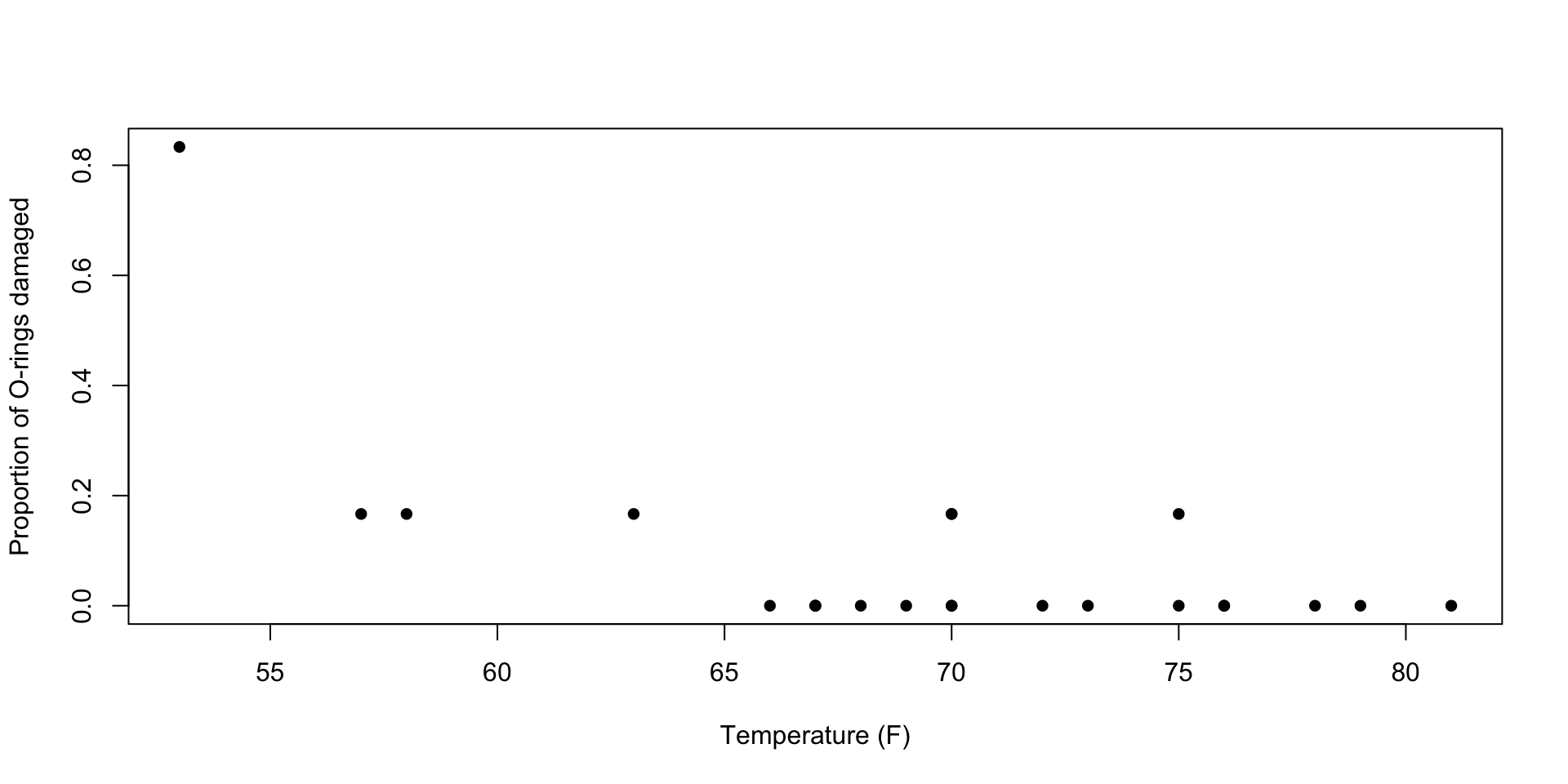
On January 28, 1986, the Challenger space shuttle suffered an accident shortly after launch, killing all crew members on board. An investigation suspected that damage to a set of critical parts called O-rings caused the disaster. It is believed that the damage is related to the temperature at launch time. The following data summarize data on O-rings for 23 shuttle missions.
Example: Challenger disaster
This plot visualizes the empirical proportion of damaged O-rings for each mission:

Example: Challenger disaster
The glm() function can be used to fit generalized linear models including logistic regression models. The family argument is used to specify the distribution of the response variable (in this case, binomial for a logistic rgression).
orings_res <- glm((damaged > 0) ~ temperature, data = orings, family = binomial)
summary(orings_res)
Call:
glm(formula = (damaged > 0) ~ temperature, family = binomial,
    data = orings)

Coefficients:
            Estimate Std. Error z value Pr(>|z|)
(Intercept)  15.0429     7.3786   2.039   0.0415 *
temperature  -0.2322     0.1082  -2.145   0.0320 *
---
Signif. codes:  0 '***' 0.001 '**' 0.01 '*' 0.05 '.' 0.1 ' ' 1

(Dispersion parameter for binomial family taken to be 1)

    Null deviance: 28.267  on 22  degrees of freedom
Residual deviance: 20.315  on 21  degrees of freedom
AIC: 24.315

Number of Fisher Scoring iterations: 5
Example: Challenger disaster
Here, our estimate of \(\beta_0\) is \(\widehat{\beta}_0=15.04\) and our estimate of \(\beta_1\) is \(\widehat{\beta}_1=-.23\).
We can interpret \(\beta_1\) as follows: for each additional degree of ambient temperature, the log-odds of experiencing an O-ring failure decreases by \(.23\).
In other words, the odds changes by a factor of \(\exp(.23)\approx.79\) as temperature increases by one degree.
Note that the \(p\)-value for \(\beta_1\) is significant at the \(.05\) level, suggesting that we can reject the null hypothesis that \(\beta_1=0\) (that temperature is not associated with O-ring failure).
Example: Challenger disaster
We can use many of the functions we used with lm objects, including:
fitted()returns the predicted probabilities for a logistic regressionpredict()can be used to generate predictionsplot()returns a series of diagnostic plotsresiduals()returns residuals–not that these are not usually the typical observed minus predicted residuals.anova()can be used to assess the model fit forglmobjects.
Example: Challenger disaster
         1          2          3          4          5          6          7
0.93924781 0.85931657 0.82884484 0.60268105 0.43049313 0.37472428 0.37472428
         8          9         10         11         12         13         14
0.37472428 0.32209405 0.27362105 0.22996826 0.22996826 0.22996826 0.22996826
        15         16         17         18         19         20         21
0.15804910 0.12954602 0.08554356 0.08554356 0.06904407 0.06904407 0.04454055
        22         23
0.03564141 0.02270329
Example: Challenger disaster
base_res <- glm((damaged > 0) ~ 1, data = orings, family = binomial)
anova(orings_res, base_res, test = "F")
Analysis of Deviance Table
Model 1: (damaged > 0) ~ temperature
Model 2: (damaged > 0) ~ 1
Resid. Df Resid. Dev Df Deviance F Pr(>F)
1 21 20.315
2 22 28.267 -1 -7.952 7.952 0.004804 **
---
Signif. codes: 0 '***' 0.001 '**' 0.01 '*' 0.05 '.' 0.1 ' ' 1Analysis of Variance
The analysis of variance or ANOVA is a collection of statistical methods used to compare two or more groups to assess the differences between group means.
The simplest ANOVA provides a test of whether two or more population means are equivalent. As such the ANOVA is a generalization of the two sample \(t\)-test.
ANOVA is typically said to be introduced by Ronald Fisher, who applied the method to study the variation in crop yield related to different fertiliser treatments.
One-way ANOVA
One-way ANOVA or single-factor ANOVA is used to compare two or more population means. Let \(I\) be the number of groups/populations and \(\mu_I\) to be the population mean of the response of interest for group \(I\).
Hypotheses:
- \(H_0:\mu_1=\ldots=\mu_I\)
- \(H_a: \text{at least two of the means are different}\)
Assumptions:
- The population distributions are all normal with the same variance \(\sigma^2\).
Test Statistic
The \(F\) test is commonly used to compare the causes of the total variation. In particular, the \(F\) test statistic is defined as
\[F=\frac{\text{variance between groups}}{\text{variance within groups}}\]
If \(F\) is large, then there may be evidence to reject the hypothesis that the group means are all equal.
Test Statistic
\[F=\frac{\text{variance between groups}}{\text{variance within groups}}=\frac{ \text{Mean Square for Treatments}}{\text{Mean Square for Error}}\]
In a balanced design, where each group has the same number of \(J\) samples, and \(X_{i, j}\) denotes the \(j\)th measurement from group \(i\), the mean square terms have the following formulas:
\[\text{Mean Square for Treatments}=\frac{J}{I-1}\sum_i(\overline{X}_i-\overline{X}_{\cdot\cdot})^2\]
where \(\overline{X}_i\) is the sample group mean and \(\overline{X}_{\cdot\cdot}\) is the overall sample mean.
\[\text{Mean Square for Error}=\frac{S_1^2+S_2^2+\cdots+S_I^2}{I}\]
Example: PlantGrowth
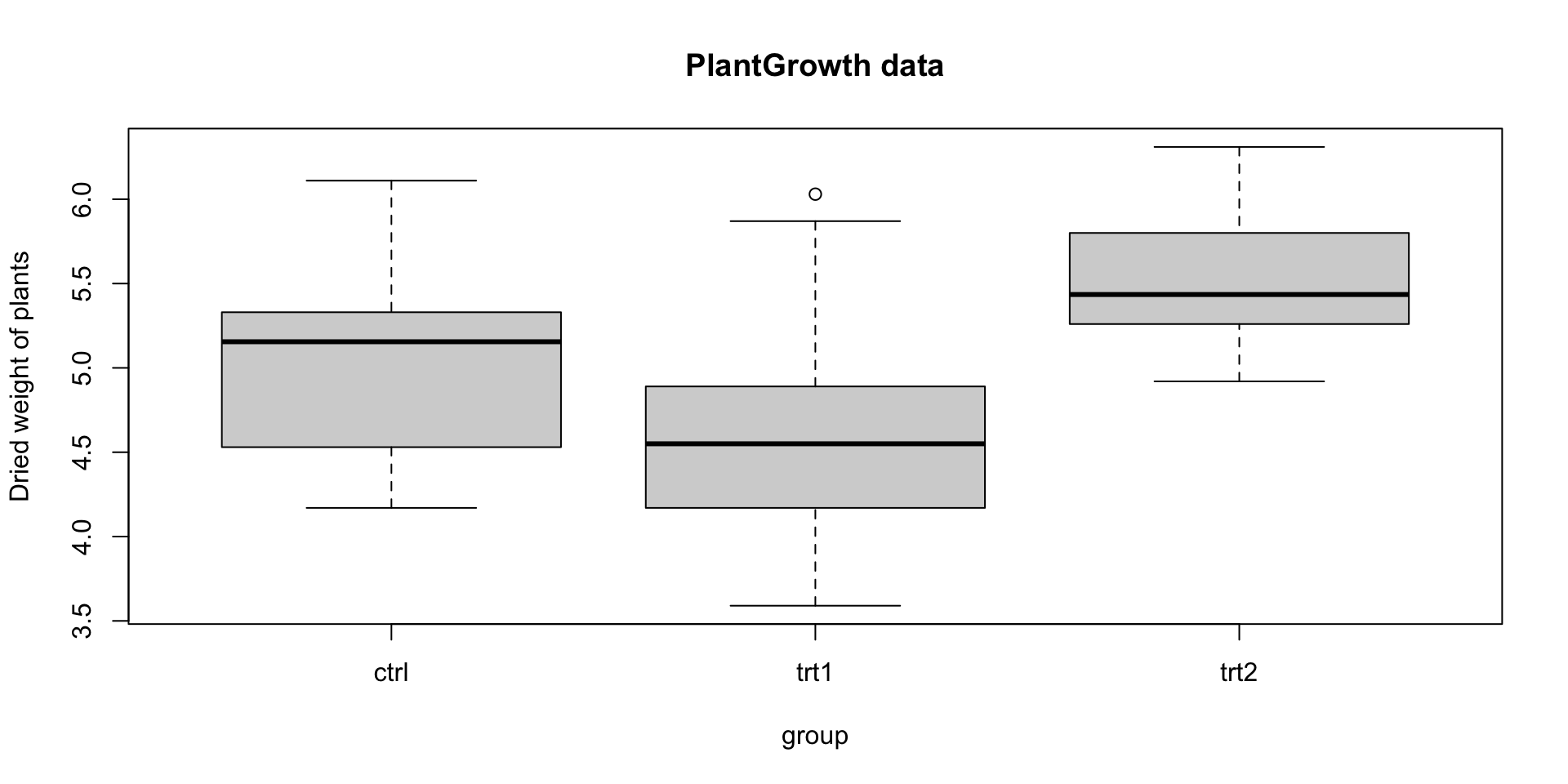
The PlantGrowth data provides results from an experiment comparing plant growth under a control and two different treatment conditions.

Example: PlantGrowth
Obtaining a \(p\)-value with an \(F\)-test statistic
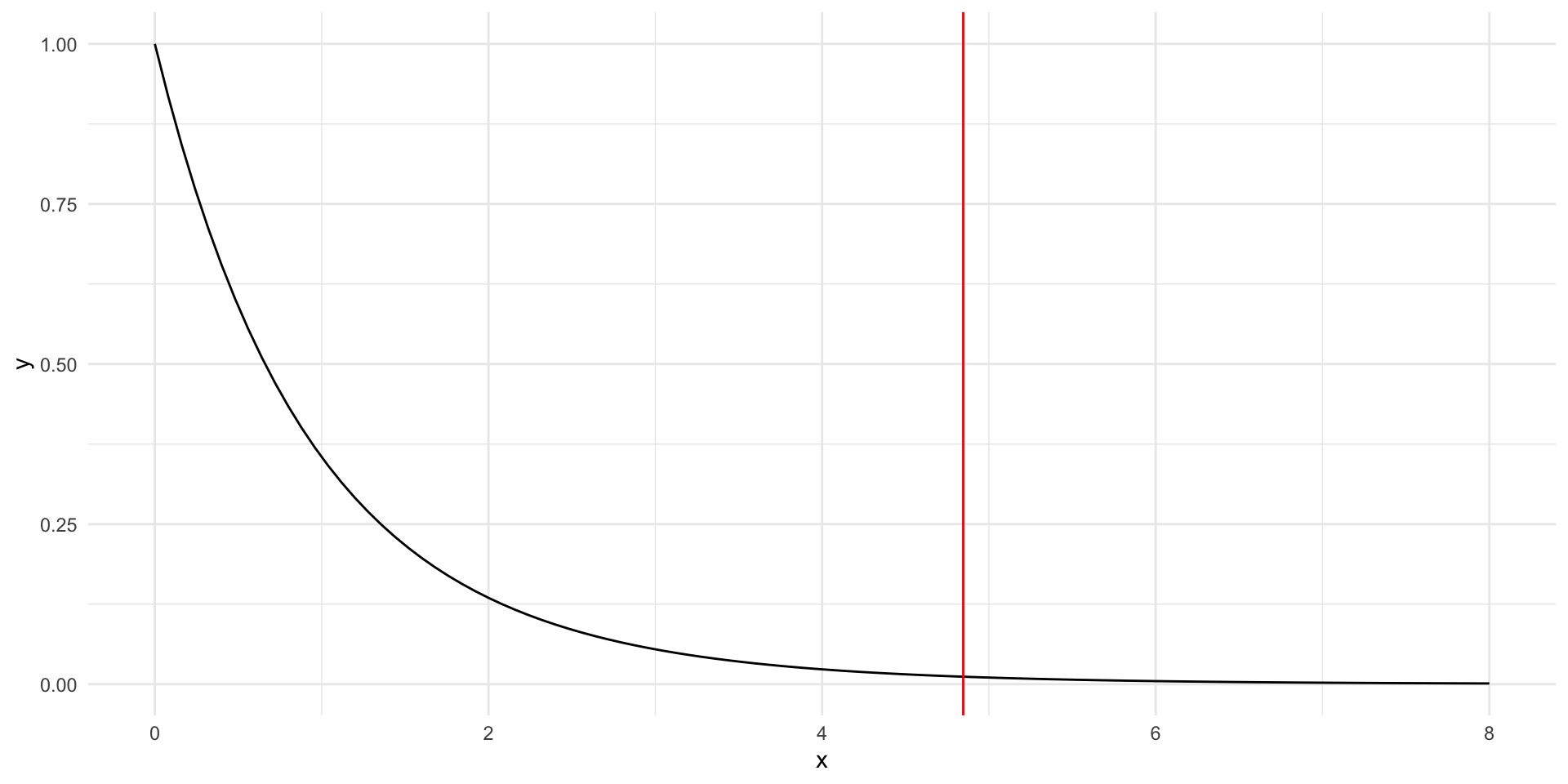
When \(H_0\) is true, \(F\) follows an \(F\)-distribution with \(\nu_1=I-1\) and \(\nu_2=I(J-1)\).

The \(F\)-distribution
The \(F\) distribution has two parameters:
- numerator degrees of freedom \(\nu_1\)
- denominator degrees of freedom \(\nu_2\)
The \(F\) distribution was derived as the ratio of (scaled) chi-square random variables and is frequently used to model the null distribution of test statistics.
\[F = \frac{U_1/d_1}{U_2/d_2}\]
where \(U_1\) is chi-square with \(d_1\) degrees of freedom, \(U_2\) is chi-square with \(d_2\) degrees of freedom, and \(U_1\) and \(U_2\) are independent.
Example: emails
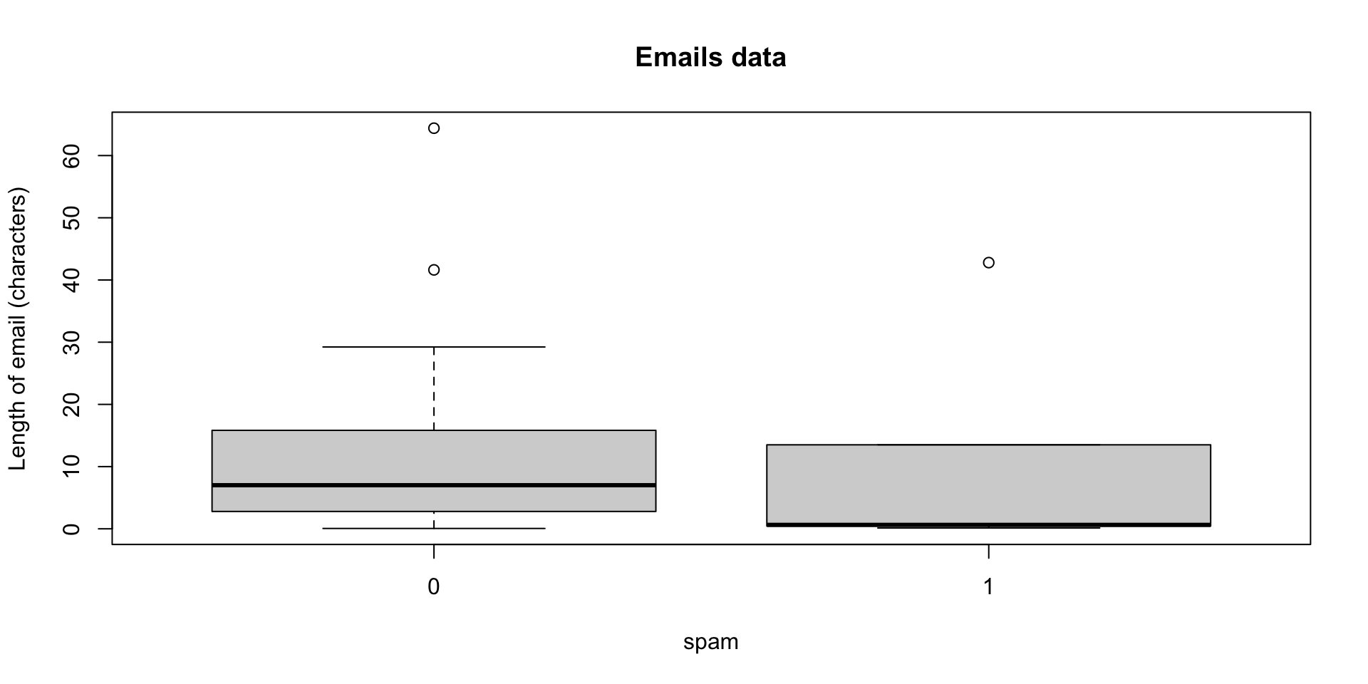
The emails data provides information on emails categorized as spam and non-spam.

Example: emails
The General Linear \(F\)-test
In general, the anova() function can be used to test the fit of a model for sample data.
For a simple linear regression case, the \(F\) test can be used to compare a full model of the form
\[y_i = (\beta_0+\beta_1x_{i1})+\epsilon_i\]
with a reduced model:
\[y_i=\beta_0+\epsilon_i\] ## The General Linear \(F\)-test
Hypotheses:
- \(H_0:y_i=\beta_0+\epsilon_i\)
- \(H_a: y_i=\beta_0+\beta_1x_{i1}+\epsilon_i\)
The General Linear \(F\)-test
Let \(p_{full}\) be the number of parameters in the full model and \(p_{reduced}\) be the number of parameters in the reduced model.
Let \(SSE_{full}\) and \(SSE_{reduced}\) be the sum of squared errors for the full and reduced models, respectively.
\[ F = \frac{(SSE_{reduced}-SSE_{full})/(p_{full}-p_{reduced})}{SSE_{full}/p_{full}} \]
Then \(F\) follows an \(F\) distribution with \(p_{full}-p_{reduced}\) and \(p_{full}\) degrees of freedom.
Example: mtcars
Example: mtcars
Note that this is equivalent to the Wald test for the coefficient for wt in the univariate case:
Call:
lm(formula = mpg ~ wt, data = mtcars)

Residuals:
    Min      1Q  Median      3Q     Max
-4.5432 -2.3647 -0.1252  1.4096  6.8727

Coefficients:
            Estimate Std. Error t value Pr(>|t|)
(Intercept)  37.2851     1.8776  19.858  < 2e-16 ***
wt           -5.3445     0.5591  -9.559 1.29e-10 ***
---
Signif. codes:  0 '***' 0.001 '**' 0.01 '*' 0.05 '.' 0.1 ' ' 1

Residual standard error: 3.046 on 30 degrees of freedom
Multiple R-squared:  0.7528,    Adjusted R-squared:  0.7446
F-statistic: 91.38 on 1 and 30 DF,  p-value: 1.294e-10
The General Linear \(F\)-test
More generally the \(F\)-test can be used to test sets of nested models, when a reduced model can be compared with a full model.
Hypotheses:
- \(H_0: \text{reduced model true}\)
- \(H_a: \text{full model fits better}\)
Example: mtcars
Analysis of Variance Table

Response: mpg
          Df Sum Sq Mean Sq F value    Pr(>F)
hp         1 678.37  678.37 100.862 5.987e-11 ***
wt         1 252.63  252.63  37.561 1.120e-06 ***
Residuals 29 195.05    6.73
---
Signif. codes:  0 '***' 0.001 '**' 0.01 '*' 0.05 '.' 0.1 ' ' 1
When we have more than one explanatory variable, the \(F\)-test is different from the univariate Wald test.
Example: mtcars
Call:
lm(formula = mpg ~ hp + wt, data = mtcars)

Residuals:
   Min     1Q Median     3Q    Max
-3.941 -1.600 -0.182  1.050  5.854

Coefficients:
            Estimate Std. Error t value Pr(>|t|)
(Intercept) 37.22727    1.59879  23.285  < 2e-16 ***
hp          -0.03177    0.00903  -3.519  0.00145 **
wt          -3.87783    0.63273  -6.129 1.12e-06 ***
---
Signif. codes:  0 '***' 0.001 '**' 0.01 '*' 0.05 '.' 0.1 ' ' 1

Residual standard error: 2.593 on 29 degrees of freedom
Multiple R-squared:  0.8268,    Adjusted R-squared:  0.8148
F-statistic: 69.21 on 2 and 29 DF,  p-value: 9.109e-12
Example: mtcars
We can explicitly specify the full and reduced models:
my_lm_full <- lm(mpg ~ hp + wt, data = mtcars)
my_lm_reduced <- lm(mpg ~ 1, data = mtcars)
anova(my_lm_full, my_lm_reduced)
Analysis of Variance Table
Model 1: mpg ~ hp + wt
Model 2: mpg ~ 1
Res.Df RSS Df Sum of Sq F Pr(>F)
1 29 195.05
2 31 1126.05 -2 -931 69.211 9.109e-12 ***
---
Signif. codes: 0 '***' 0.001 '**' 0.01 '*' 0.05 '.' 0.1 ' ' 1Other hypothesis tests
Fisher’s exact test
Agresti (1990): A British woman claimed to be able to distinguish whether milk or tea was added to the cup first. To test, she was given 8 cups of tea, in four of which milk was added first. The null hypothesis is that there is no association between the true order of pouring and the woman’s guess. The alternative that there is a positive association (that the odds ratio is greater than 1).
Fisher’s exact test
TeaTasting <-
  matrix(c(3, 1, 1, 3),
         nrow = 2,
         dimnames = list(Guess = c("Milk", "Tea"),
                         Truth = c("Milk", "Tea")))
fisher.test(TeaTasting, alternative = "greater")
    Fisher's Exact Test for Count Data

data:  TeaTasting
p-value = 0.2429
alternative hypothesis: true odds ratio is greater than 1
95 percent confidence interval:
 0.3135693       Inf
sample estimates:
odds ratio
  6.408309